
A Comprehensive Guide to the Polynomial Commitment Protocol Brakedown in FOAKS
TechFlow Selected TechFlow Selected
A Comprehensive Guide to the Polynomial Commitment Protocol Brakedown in FOAKS
If cryptographers had not discovered the connection between tensor products and polynomial evaluations, it would have been difficult for the polynomial commitment scheme Brakedown to emerge, making it impossible for Orion based on Brakedown and FOAK to exist.
Authors: Kang Shuiyue, CEO of Fox Tech; Meng Xuanji, Chief Scientist at Fox Tech
Preface: If cryptographers had not discovered the connection between tensor products and polynomial evaluations, it would have been difficult for the polynomial commitment protocol Brakedown to emerge, making impossible the development of Orion based on Brakedown and the entirely new fast algorithms such as FOAKS.
In many zero-knowledge proof systems relying on polynomial commitments, different commitment protocols are used. According to Justin Thaler from a16z in his August 2022 article "Measuring SNARK performance: Frontends, backends, and the future," although Brakedown has relatively large proof sizes, it is undoubtedly the fastest polynomial commitment protocol available today.
FRI, KZG, and Bulletproof are more common polynomial commitment protocols, but speed remains their bottleneck. Algorithms like Plonky adopted by zkSync, Plonky 2 used by Polygon zkEVM, and Ultra-Plonk employed by Scroll are all based on KZG polynomial commitments. The prover involves extensive FFT computations and MSM operations to generate polynomials and commitments—both imposing significant computational overhead. Although MSM can potentially benefit from multi-threaded acceleration, it requires substantial memory and remains slow even under high parallelism. Large-scale FFTs heavily depend on frequent shuffling of data during algorithm execution, making distributed acceleration across computing clusters extremely challenging.
It is precisely due to the emergence of the faster polynomial commitment protocol Brakedown that the complexity of these operations has been significantly reduced.
FOAKS (Fast Objective Argument of Knowledge) is a zero-knowledge proof system framework proposed by Fox Tech, built upon Brakedown. FOAKS further reduces FFT computations compared to Orion, aiming ultimately to eliminate FFT altogether. Additionally, FOAKS introduces a novel and highly sophisticated recursive proof mechanism to reduce proof size. The advantage of the FOAKS framework lies in achieving linear proving time while maintaining small proof sizes, making it particularly suitable for applications in zkRollup scenarios.
Below, we will detail the polynomial commitment protocol Brakedown used in FOAKS.
In cryptography, a commitment protocol allows a prover to commit to a secret value, generating a public commitment value that satisfies two properties: binding (bindingness) and hiding (hidingness). Later, the committer opens this commitment and sends the message to the verifier to validate the correspondence between the commitment and the message. This functionality shares similarities with hash functions, but commitment schemes often rely on mathematical structures from public-key cryptography. A polynomial commitment is a type of commitment scheme where the committed value is a polynomial. Furthermore, polynomial commitment protocols include algorithms that allow evaluation at given points along with proofs, making them important cryptographic primitives and core components of many zero-knowledge proof systems.
In recent advances in cryptography, the discovery of the relationship between tensor products and polynomial evaluations has led to a series of related polynomial commitment protocols, with Brakedown being a representative example.
Before diving into the details of Brakedown, some foundational knowledge must first be introduced: linear codes, collision-resistant hash functions, Merkle trees, tensor product operations, and the tensor product representation of polynomial evaluations.
First, linear codes. A linear code of message length k and codeword length n is a linear subspace C ⊆ Fⁿ, such that there exists an injective mapping from messages to codewords called encoding, denoted EC: Fᵏ → C. Any linear combination of codewords is still a valid codeword. The distance between two codewords u and v is their Hamming distance, denoted Δ(u, v).
The minimum distance is d = min_{u,v} Δ(u, v). Such a code is denoted as an [n, k, d] linear code, with relative distance d/n.
Next, collision-resistant hash functions and Merkle trees.
Let H: {0, 1}²ˡ → {0, 1}ˡ denote a hash function. A Merkle tree is a special data structure enabling commitment to 2ᵈ messages, producing a single hash value h. To open any message, d+1 hash values are required.
A Merkle tree can be represented as a binary tree of depth d, where L message elements m₁, m₂, ..., mₗ correspond to the leaves. Each internal node is computed by hashing its two child nodes. To reveal message mᵢ, one must disclose the path from mᵢ to the root.
We use the following notation:
-
h ← Merkle.Commit(m₁, ..., mₗ)
-
(mᵢ, πᵢ) ← Merkle.Open(m, i)
-
{0, 1} ← Merkle.Verify(πᵢ, mᵢ, h)
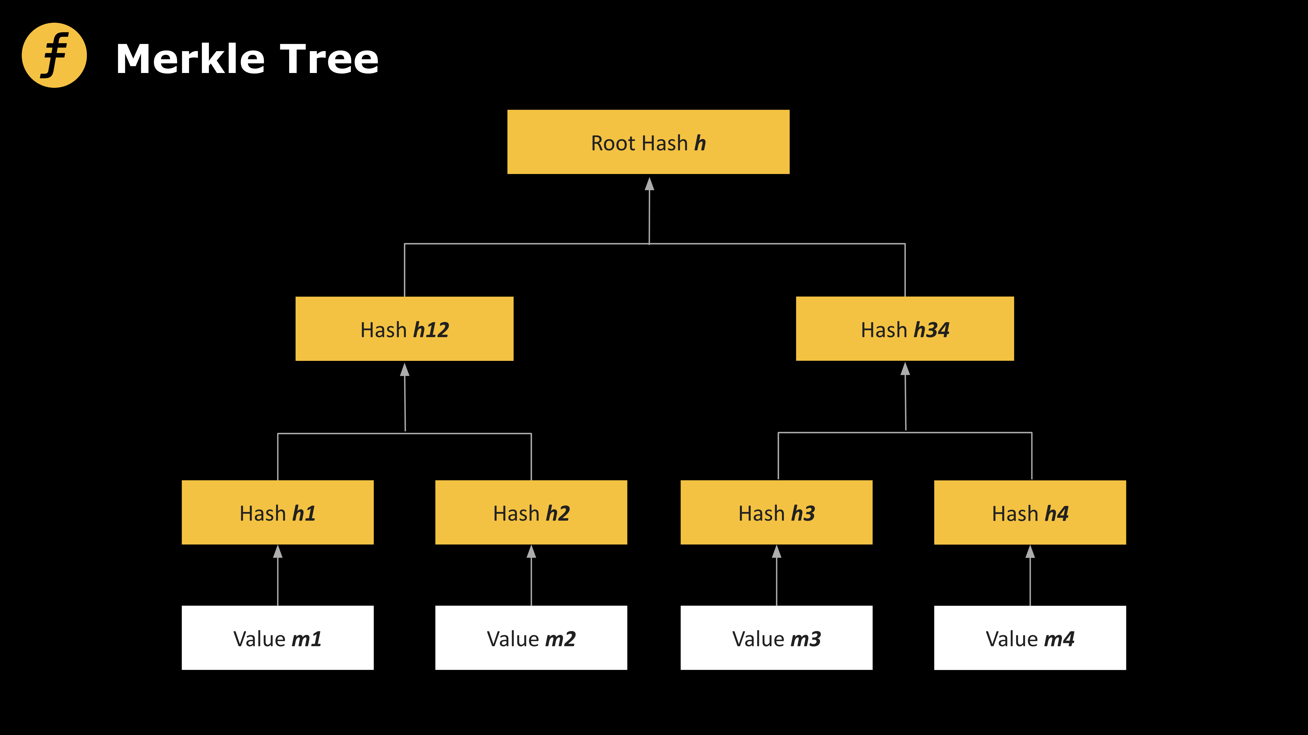
Figure 1: Merkle Tree
We also need to understand how tensor product operations work. Mathematically, tensors extend vectors and matrices into higher-dimensional spaces and are important research objects. A full discussion of tensors goes beyond the scope of this article; here we only introduce tensor products of vectors and matrices.
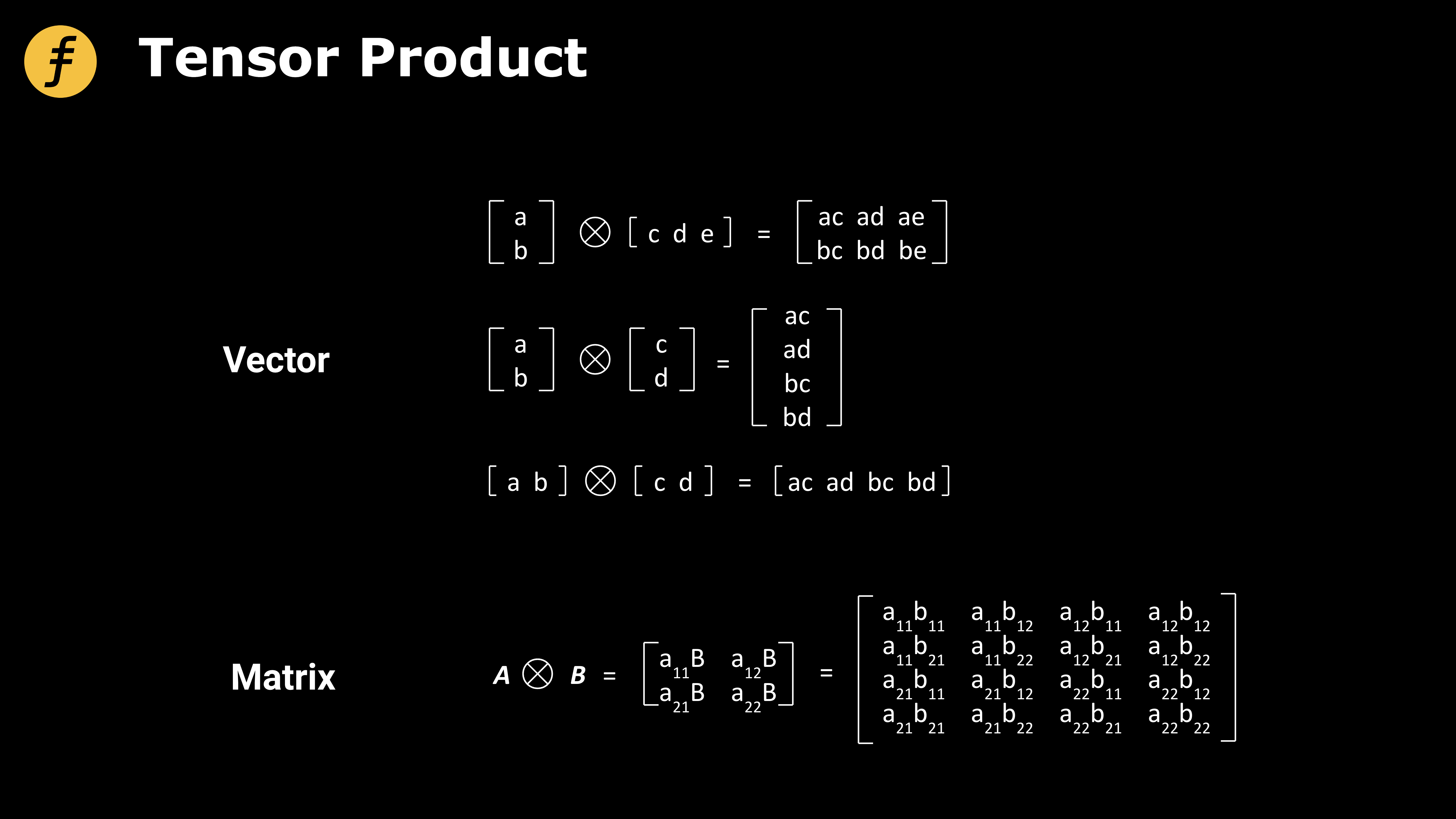
Figure 2: Tensor Product Operation for Vectors and Matrices
Next, we need to know about the tensor product representation of polynomial evaluations.
As mentioned in [GLS+], polynomial evaluations can be expressed in the form of tensor products. Here, we consider commitments to multilinear polynomials.
Specifically, given a polynomial, its evaluation at vector x₀, x₁, ..., x_{logN−1} can be written as:
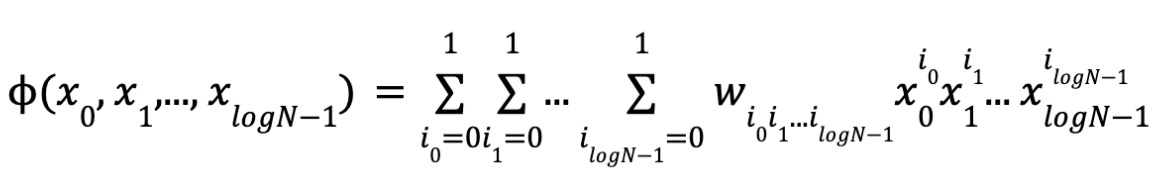
By definition of multilinearity, each variable appears with degree 0 or 1. Thus, there are N monomials and coefficients, and logN variables. Let
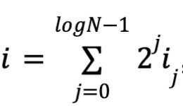
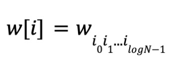
where i₀i₁...i_{logN−1} is the binary representation of i. Let w represent the polynomial coefficients,
Similarly, define
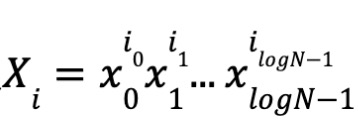
Let
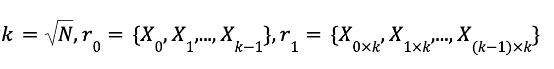
Thus, X = r₀ ⊗ r₁.
Therefore, polynomial evaluation can be expressed using tensor products: ϕ(x₀, x₁, ..., x_{logN−1}) = ⟨w, r₀ ⊗ r₁⟩.
Finally, let us examine the Brakedown procedure used in FOAKS and Orion [XZS 22].
First, PC.Commit divides the polynomial coefficient w into a k×k matrix and encodes it (see "Preliminaries" section on linear codes), denoted as C₂. Then, a Merkle tree is constructed for each column C₂[:, i] of C₂. Another Merkle tree is then built over the roots of these column-wise Merkle trees, forming the final commitment.
In the evaluation proof computation, two aspects must be verified: proximity and consistency. Proximity ensures that the committed matrix is sufficiently close to an encoded codeword. Consistency guarantees y = ⟨w, r₀ ⊗ r₁⟩.
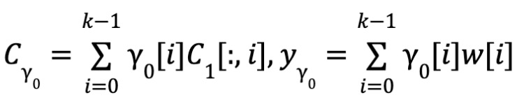
Proximity Test: The proximity test consists of two steps. First, the verifier sends a random vector Y₀ ∈ Fᵏ to the prover. The prover computes the inner product Y₀ with C₁—that is, computes a linear combination of the rows of C₁ using components of Y₀ as coefficients. Due to the linearity of the code, C_{Y₀} is a codeword of Y_{Y₀}. Then, the prover proves that C_{Y₀} was indeed computed from the committed codeword. To do so, the verifier randomly selects t columns, and the prover opens those columns and provides Merkle tree proofs. The verifier checks whether the inner products of these columns with Y₀ match the corresponding entries in C_{Y₀}. As shown in [BCG 20], if the linear code used has constant relative distance, then the committed matrix is overwhelmingly likely to be close to a valid codeword (overwhelming probability means the probability of the negation is negligible).
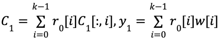
Consistency Test: The consistency test follows a similar flow to the proximity test. The difference is that instead of using a random vector Y₀, r₀ is directly used for the linear combination. Similarly, c₁ is a linear code of message y₁, and we have ϕ(x) = ⟨y₁, r₁⟩. As proved in [BCG 20], passing the consistency test implies that if the committed matrix is close to a codeword, then y = ϕ(x) holds with overwhelming probability.
In pseudocode form, the Brakedown protocol proceeds as follows:
Public input: The evaluation point X, parsed as a tensor product X = r₀ ⊗ r₁;
Private input: The polynomial ϕ, whose coefficients are denoted by w.
Let C be the [n, k, d]-linear code, EC: Fᵏ → Fⁿ be the encoding function, N = k × k. If N is not a perfect square, pad it to the next perfect square. We use Python-style notation mat[:, i] to select the i-th column of a matrix mat.
-
function PC.Commit(ϕ):
-
Parse w as a k×k matrix. The prover locally computes the tensor code encoding C₁, C₂, where C₁ is a k×n matrix and C₂ is an n×n matrix.
-
for i ∈ [n] do
-
Compute the Merkle tree root Rootᵢ = Merkle.Commit(C₂[:, i])
-
Compute a Merkle tree root R = Merkle.Commit([Root₀, ..., Root_{n−1}]), and output R as the commitment.
-
function PC.Prover(ϕ, X, R)
-
The prover receives a random vector Y₀ ∈ Fᵏ from the verifier.
-
Proximity
-
Consistency
-
Prover sends C₁, y₁, C₀, y₀ to the verifier.
-
Verifier randomly samples t indices from [n] as an array Î and sends it to the prover.
-
for idx ∈ Î do
-
Prover sends C₁[:, idx] and the Merkle tree proof of Root_idx for C₂[:, idx] under R to the verifier.
-
function PC.VERIFY_EVAL(πₓ, X, y=ϕ(X), R)
-
Proximity: ∀idx ∈ Î, C_{Y₀}[idx] == ⟨Y₀, C₁[:, idx]⟩ and EC(Y_{Y₀}) == C_{Y₀}
-
Consistency: ∀idx ∈ Î, C₁[idx] == ⟨r₀, C₁[:, idx]⟩ and EC(y₁) == C₁
-
y == ⟨r₁, y₁⟩
-
∀idx ∈ Î, EC(C₁[:, idx]) is consistent with Root_idx, and Root_idx’s Merkle tree proof is valid.
-
Output accept if all conditions above hold. Otherwise output reject.
Conclusion: Polynomial commitments are a critically important class of cryptographic protocols widely used in various cryptographic systems, especially zero-knowledge proof systems. This article provides a detailed explanation of the Brakedown polynomial commitment protocol and its underlying mathematics. As a key foundational component of FOAKS, Brakedown plays a vital role in enhancing the practical performance of FOAKS implementations.
References
-
[GLS+]: Alexander Golovnev, Jonathan Lee, Srinath Setty, Justin Thaler, and Riad S. Wahby. Brakedown: Linear-time and post-quantum snarks for r 1 cs. Cryptology ePrint Archive. https://ia.cr/2021/1043.
-
[XZS 22]: Xie T, Zhang Y, Song D. Orion: Zero knowledge proof with linear prover time[C]//Advances in Cryptology–CRYPTO 2022: 42nd Annual International Cryptology Conference, CRYPTO 2022, Santa Barbara, CA, USA, August 15–18, 2022, Proceedings, Part IV. Cham: Springer Nature Switzerland, 2022: 299-328. https://eprint.iacr.org/2022/1010
-
[BCG 20]: Bootle, Jonathan, Alessandro Chiesa, and Jens Groth. "Linear-time arguments with sublinear verification from tensor codes." Theory of Cryptography: 18th International Conference, TCC 2020, Durham, NC, USA, November 16–19, 2020, Proceedings, Part II 18. Springer International Publishing, 2020.
-
Justin Thaler from A16z crypto, Measuring SNARK performance: Frontends, backends, and the future https://a16z crypto.com/measuring-snark-performance-frontends-backends-and-the-future/
-
Introduction to tensor products: https://blog.csdn.net/chenxy_bwave/article/details/127288938
Join TechFlow official community to stay tuned
Telegram:https://t.me/TechFlowDaily
X (Twitter):https://x.com/TechFlowPost
X (Twitter) EN:https://x.com/BlockFlow_News