




STARK: Polynomial Proofs
TechFlow Selected TechFlow Selected
STARK: Polynomial Proofs
How does this new zero-knowledge proof actually work?
 Navigating Web3 tides with focused insights
Many people have heard of ZK-SNARKs, a general and succinct zero-knowledge proof technology applicable to various scenarios ranging from verifiable computation to privacy-preserving cryptocurrencies. However, you might not yet know that ZK-SNARKs now have a new sibling: ZK-STARKs. The "T" here stands for "transparent," meaning ZK-STARKs solve a major drawback of ZK-SNARKs—namely their reliance on a "trusted setup." ZK-STARKs also rely on simpler cryptographic assumptions, avoid the use of elliptic curves, pairings, and the knowledge-of-exponent assumption, and are entirely based on hashing and information theory. This means they remain secure even against attackers using quantum computers.
Of course, this comes at a cost: proof size increases from 288 bytes (B) to several hundred kilobytes (KB). While this trade-off may not always be worthwhile, in certain contexts—especially blockchain applications requiring high trust minimization—it could be well justified. And should elliptic curve cryptography be broken or quantum computers become reality, the switch would undoubtedly be worth it.
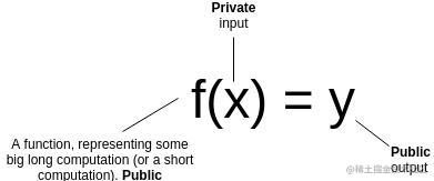
So how does this new kind of zero-knowledge proof actually work? First, let’s revisit what succinct, general-purpose zero-knowledge proofs aim to achieve. Suppose you have a (public) function f, a (private) input x, and a (public) input y. You want to prove that you know an x such that f(x) = y, without revealing what x is (for example, proving you know the password to a safe without disclosing the password itself). Additionally, for the proof to be succinct, you want verification to be significantly faster than computing f directly.
Let’s consider a few examples:
-
f is a computation taking two weeks on a regular computer but only two hours on a data center. You send the task (the code implementing f) to the data center; it computes the result y and returns a proof. You verify the proof in milliseconds and can be confident y is correct.
-
You have an encrypted transaction structured as “X1 is my old balance, X2 is your old balance, X3 is my new balance, X4 is your new balance.” You want to prove this transaction is valid (i.e., all balances are non-negative and my decrease equals your increase). Here, x could be a pair of private keys, f a function that decrypts the transaction with those keys, checks validity, and returns 1 if valid, 0 otherwise. Then y must be 1.
-
You’re downloading the latest block of an Ethereum-like blockchain and want to prove it's valid and extends a chain where every prior block is valid. You ask a known full node to provide such a proof. Here, x is the entire (or partial) blockchain, f processes each block sequentially verifying validity and outputs the previous block’s hash, and y is the hash of the block you just downloaded.
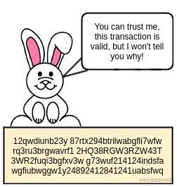
So what makes these cases difficult? It turns out that zero-knowledge (i.e., privacy) is (relatively!) easy to achieve. There are multiple ways to convert any computation into something akin to a graph three-coloring problem, where a valid coloring corresponds to a solution of the original problem, and then use classical zero-knowledge protocols to prove knowledge of a valid coloring without revealing it. Matthew Green’s excellent 2014 article explains the details.
The harder challenge is succinctness. Intuitively, proving computational facts succinctly is hard because computation is extremely fragile. If you have a long, complex calculation, changing even a single bit midway often leads to a completely different outcome. Thus, it’s hard to imagine how one could verify correctness via random sampling of the computation trace, since it's easy to miss that “one evil bit.” Yet, through sophisticated mathematics, it turns out this is possible.
The high-level intuition behind these protocols draws from techniques like those used in erasure coding, which make data fault-tolerant. If you have some data and encode it as points on a line, selecting four points suffices so that any two can reconstruct the line and thus recover the other two. More powerfully, you can encode data as a degree-1,000,000 polynomial and sample 2,000,000 points; any 1,000,001 points can reconstruct the original data and hence all others. Any small change in the original data alters at least 1,000,000 points. The algorithms described here heavily leverage polynomials in this way to achieve error amplification.
A Simple Example
Suppose you want to prove you have a polynomial P such that for all integers x from 1 to 1 million, P(x) is an integer satisfying 0 <= P(x) <= 9. This is a simple instance of a common "range check." You might use such a check to verify account balances remain positive after transactions. If instead 1 <= P(x) <= 9, this could help validate a correct Sudoku solution.
The "traditional" way to verify this would be to evaluate P(x) at all 1,000,000 points and check each value individually. But we’d like to know whether we can construct a proof that can be verified in far fewer steps. Simply randomly sampling a few values won’t work—there could always be a malicious prover who constructs a P that satisfies the condition at 999,999 points but fails at one, and random sampling would likely miss it. So what can we do?
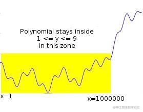
Let’s reframe the problem mathematically. Let C(x) be a constraint-checking polynomial that equals zero if 0 <= x <= 9 and nonzero otherwise. A simple construction is C(x) = x * (x-1) * (x-2) * ... * (x-9).
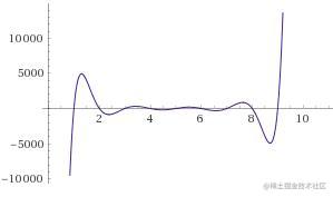
Now the problem becomes: prove you know P such that C(P(x)) = 0 for all x from 1 to 1,000,000. Let Z(x) = (x-1) * (x-2) * ... * (x-1,000,000). A known mathematical fact is that any polynomial vanishing at all these points must be divisible by Z(x). So we reformulate again: prove you know P and D such that C(P(x)) = Z(x) * D(x) for all x. (Note: computing D(x) given a valid C(P(x)) isn't too hard—you can use polynomial long division or faster FFT-based algorithms.) Now we've transformed the original statement into a mathematically cleaner and more provable form.
How do we prove this? Imagine a three-step interaction between a prover and a verifier:
- Prover sends some information
- Verifier sends a challenge
- Prover responds with more information
First, the prover commits to (i.e., builds a Merkle tree and sends its root hash to the verifier) the values of P(x) and D(x) for all x from 1 to 1 billion (yes, one billion). This includes 1 million points where 0 <= P(x) <= 9 and 999 million potentially arbitrary points.
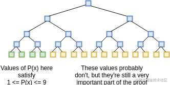
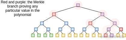
We assume the verifier already knows Z(x) at all these points; in this scheme, Z(x) acts like a public verification key everyone must know in advance (a client might not store Z(x) fully but only its Merkle root, requiring the prover to supply Merkle branches for queried Z(x) values—or Z(x) might be efficiently computable on-the-fly for any x). After receiving the commitment (Merkle root), the verifier randomly selects 16 values of x between 1 and 1 billion and requests Merkle branches for P(x) and D(x) at those points. The prover supplies them, and the verifier checks:
-
The branches match the previously provided Merkle root
-
C(P(x)) equals Z(x) * D(x) in all 16 cases
We know this proof has completeness—if you truly know a valid P(x), compute D(x) correctly, and construct the proof properly, all 16 checks will pass. But what about soundness?
That is, if a malicious prover provides an invalid P(x), what’s the minimum chance they’ll get caught? We analyze as follows: C(P(x)) is a degree-1,000,000 polynomial, so its degree is at most 10,000,000.
Generally, two distinct degree-N polynomials intersect in at most N points. Hence, any polynomial differing from Z(x)*D(x) must differ at at least 990,000,000 points. Therefore, even a single check has a 99% chance of catching a bad P(x); with 16 checks, the detection probability rises to 1 - 10^-32—making it as hard to cheat as finding a hash collision.
What did we just accomplish? We used polynomials to "amplify" errors in bad solutions, transforming a problem requiring one million direct checks into a verification protocol where even one check detects errors with 99% probability.
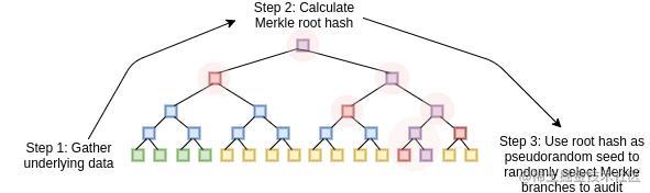
We can turn this three-step protocol into a non-interactive proof using the Fiat-Shamir heuristic, allowing a prover to broadcast a proof verifiable by anyone. The prover first builds a Merkle tree of P(x) and D(x) values, computes its root, and uses the root itself as a source of randomness to determine which branches to reveal. The prover then broadcasts both the Merkle root and the selected branches as the proof. All computation happens on the prover side. By deriving the Merkle root from the data and using it to pseudo-randomly select audit paths, we effectively simulate an interactive verifier.
A malicious prover without a valid P(x) can only try to repeatedly construct proofs until they luckily find a Merkle root whose corresponding branches pass verification. But with soundness around 1 - 10^-32 (i.e., any fake proof has less than a 10^-32 chance of passing), this could take billions of years.
Going Deeper
To illustrate the power of this technique, let’s do something unusual: prove you know the millionth Fibonacci number. We’ll do this by proving you know a polynomial P(x) where P(x) represents the x-th Fibonacci number. The constraint-checking polynomial now spans three coordinates: C(x1, x2, x3) = x3 - x2 - x1 (note that for all x, if P(x) follows the Fibonacci recurrence, then C(P(x), P(x+1), P(x+2)) = 0).
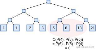
-Fibonacci-
The transformed problem becomes: verify you know P and D such that C(P(x), P(x+1), P(x+2)) = Z(x) * D(x). For each of the 16 audit points, the prover must provide Merkle branches for P(x), P(x+1), P(x+2), and D(x). The prover must also provide additional branches proving P(0) = P(1) = 1. Otherwise, the process remains unchanged.
Now, to implement this in practice, two issues remain. First, this scheme is inefficient for ordinary integers because numbers grow extremely large—for example, the millionth Fibonacci number has over 200,000 bits. To achieve practical succinctness, we need to operate not on regular integers but on finite fields—number systems obeying standard arithmetic laws like a*(b+c)=(a*b)+(a*c) and (a²-b²)=(a-b)*(a+b), but where every number occupies constant space. Proving knowledge of the millionth Fibonacci number would require a more sophisticated design implementing big-number arithmetic over finite fields.
The simplest and most common finite field is modular arithmetic: for some prime N, replace every a + b with a + b mod N, applying similar operations to subtraction and multiplication, and using modular inverses for division (e.g., if N = 7, then 3 + 4 = 0, 2 + 6 = 1, 3 * 4 = 5, 4 / 2 = 2, 5 / 2 = 6). You can learn more about such systems in my introduction to prime fields (search “prime field” on that page), or refer to Wikipedia articles on finite fields and prime fields (which may seem abstract but are manageable).
Second, you may have noticed that in my sketch of the soundness argument above, I ignored one attack: what if the attacker doesn’t submit P(x) and D(x) derived from low-degree polynomials at all? Since a valid C(P(x)) must differ from any invalid one at at least 990 million points, such attacks could be harder to catch. For instance, an attacker could generate random p for each x, compute d = C(p)/Z(x), and submit these as P(x) and D(x). These values wouldn’t come from low-degree polynomials, yet they would pass the test.
It turns out that although the tools involved are quite complex, this possibility can still be effectively prevented—and this gap is precisely where much of the mathematical innovation in STARKs lies. However, there's a limitation: while these tools can rule out commitments to data that differ significantly from any degree-1,000,000 polynomial (say, requiring changes to 20% of all values), they cannot exclude data differing in just one or two coordinates. Thus, these tools give us a proof of proximity—proving that most points on P and D lie close to such polynomials.
Therefore, despite two “catches,” constructing a proof is still sufficient. First, the verifier must perform extra checks to account for potential errors introduced by this limitation. Second, if we’re doing “boundary constraint checking” (e.g., proving P(0) = P(1) = 1 in the Fibonacci example), we need to extend the proximity proof to show not only that most points lie on a low-degree polynomial but also that these specific points (or however many we care to check) lie on it.
In the next part of this series, I’ll dive deeper into solutions for the proximity testing problem.
Join TechFlow official community to stay tuned
Telegram:https://t.me/TechFlowDaily
X (Twitter):https://x.com/TechFlowPost
X (Twitter) EN:https://x.com/BlockFlow_News
 @VitalikButerin