




Stablecoin In-Depth Research: Early Stage Focuses on Incentives, Mid-Term on Depth, Long-Term on Use Cases
2022.04.27
Share Share to X (Twitter) Navigating Web3 tides with focused insights
Share to WeChat
Share to WeiboShare to WeChat
Share by Link
Share by Image
TechFlow Selected TechFlow Selected
Stablecoin In-Depth Research: Early Stage Focuses on Incentives, Mid-Term on Depth, Long-Term on Use Cases
"Stable analysis, early focus on incentives, mid-term on depth, long-term on scenarios."
2022.04.27 - 08:41:13
算稳
Navigating Web3 tides with focused insights"Stable analysis, early focus on incentives, mid-term on depth, long-term on scenarios."
1. Non-collateralized issuance is both the definition and original sin of algorithmic stablecoins. The "death spiral" is a constant threat facing every algorithmic stablecoin project, and all their intricate designs and operations are fundamentally aimed at resisting this threat.
2. When analyzing algorithmic stablecoin projects, focus in the early stage on incentive mechanism design and yield; in the mid-term, pay attention to the depth of its liquidity pools and integration with other mainstream crypto assets; in the long run, evaluate its application scenarios and potential as a medium of exchange.
**I. Classification of Stablecoins and the Definition of Algorithmic Stablecoins**
Although cryptocurrencies are gaining increasing global recognition, most people still mentally value wealth in fiat currency due to crypto's high volatility and limited purchasing power in the real world. Thus, stablecoins pegged to fiat currencies were invented to serve as stores of value and mediums of exchange within the crypto ecosystem.
Stablecoins can be broadly categorized into three types:
1. Centralized institutions issuing fiat-pegged stablecoins backed 1:1 by fiat reserves, represented by USDC;
2. Decentralized stablecoins over-collateralized by major crypto assets such as ETH, represented by DAI;
3. Decentralized stablecoins that are neither fully collateralized nor over-collateralized by mainstream crypto assets, represented by UST and FRAX. These typically feature sophisticated mechanisms and algorithms, hence referred to as algorithmic stablecoins (Algorithmic Stablecoin).
**II. Algorithmic Stablecoins: Original Sin and Temptation**
The very definition of an algorithmic stablecoin—"non-full collateralization"—is simultaneously its inherent flaw and source of temptation for project teams.
From the project team’s perspective, because algorithmic stablecoins do not require over-collateralization (or even any collateral), the difference between the stablecoin’s market cap and the value of its backing assets approximates “pure profit” for the team—a form of “printing money out of thin air,” which is indeed an irresistible temptation.
From the user’s standpoint, the under-collateralized nature means that if all holders attempt to sell or redeem their stablecoins simultaneously, the last ones left will bear the losses from insufficient collateral. In practice, once market confidence in an algorithmic stablecoin erodes, panic and selling often escalate into a self-reinforcing “death spiral.” This collapse mechanism closely resembles historical hyperinflations of fiat currencies, such as the Nationalist government's gold yuan or Weimar Germany's mark.
Therefore, preventing a “death spiral” is the core challenge every algorithmic stablecoin team must address. Many complex and sophisticated mechanism designs are ultimately centered around this issue.
**III. Further Reflection: Why Would Users Hold Algorithmic Stablecoins?**
A “death spiral” begins only when users abandon holding the stablecoin.
Let us go deeper: What motivates users to hold algorithmic stablecoins?
Is it for value storage? Not really—if the face value is $1, why would users choose riskier algorithmic stablecoins over more reliable options like USDC or DAI for storing value?
In reality, **the primary motivation for users to hold algorithmic stablecoins today is the investment returns offered by the project team.** However, relying solely on yields to attract users makes the project resemble a Ponzi scheme—“paying old investors with funds from new ones”—which is inherently unsustainable.
Therefore, **in the long term, for algorithmic stablecoins to truly retain users, they must expand into diverse real-world applications that meet genuine user needs.** For example, fulfilling the role of a transaction medium: suppose the top 100 DApps all accept a certain algorithmic stablecoin to purchase tokens and NFTs within their ecosystems—wouldn’t users mind keeping extra of that coin in their wallets?
However, given the current state of the crypto application layer, achieving such widespread adoption is no easy task:
- On one hand, there are few high-quality application projects, many of which struggle with economic sustainability themselves;
- On the other hand, convincing quality projects to integrate requires the stablecoin itself to first reach a certain scale and stability—a classic “chicken-and-egg” problem.
Thus, a viable transitional strategy for an algorithmic stablecoin project is: in the early stages, use high yields to attract users and grow scale; as the project expands, gradually reduce yield incentives, deepen liquidity pools by linking with more stable assets (e.g., USDT, USDC, DAI), enhance the system’s capacity to handle redemptions, and aggressively build real-world use cases. When users hold the coin not for yield but for utility, the project has matured. This forms the core thesis of this article: **"Analyze algorithmic stablecoins: early on, look at incentives; mid-term, look at depth; long-term, look at use cases."**
Let us now examine prominent algorithmic stablecoin projects through this developmental lens.
**IV. Early Algorithmic Stablecoins: Failures of Pure Mechanism Design**
Early algorithmic stablecoins mainly included **AMPL, ESD, and BAC**, sharing the common trait of attempting to maintain a $1 peg purely through internal supply mechanisms—an idealistic experiment. They lacked high-yield incentives to retain early adopters, external asset collateral, or efforts toward building applications and ecosystems. Unsurprisingly, none succeeded.
**4.1 AMPL: Simple and Direct Rebase Mechanism**
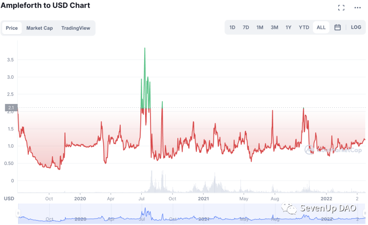
*Figure: AMPL price chart*
AMPL (Ampleforth) was among the earliest attempts at algorithmic stablecoins, implementing a rebase mechanism to adjust supply: when AMPL price > $1, tokens are proportionally minted and distributed to holders, increasing supply to push price back down; when price < $1, tokens are proportionally burned. This rebasing occurs every 8 hours, directly altering balances in users’ wallets.
The designers’ economic rationale appears straightforward: **since price is determined by supply and demand, dynamically adjusting supply should match current demand.**
However, in practice, the rebase mechanism amplified volatility by triggering FOMO: during expansions, holders gain both more tokens and rising prices, encouraging holding and attracting new capital. As long as consensus holds, market cap grows faster than inflows. Conversely, during contractions, falling prices and fewer tokens create double losses, accelerating sell-offs and deterring new capital.
Thus, **AMPL became known as a “thrilling casino.”** While it occasionally hovers near $1, its volatility far exceeds other stablecoins. With daily trading volume around $1 million, it has largely faded from public attention.
**4.2 ESD and BAC: Bond Mechanisms and Growing Systemic Deficits**
ESD (Empty Set Dollar) and BAC (Basis Cash) sought price stability not through direct supply changes, but by incentivizing users to sacrifice short-term liquidity via future rewards.
ESD pioneered the “bond mechanism.” When ESD trades above $1, users must stake ESD or ESD-USDC LP tokens to earn rewards from supply expansion—unlike AMPL, rewards aren’t “free.” When ESD trades below $1, users can buy discounted bonds. When price returns above $1, bondholders are prioritized in new token distribution, followed by stakers.
> For example: ESD trades at $0.99. A $1 face-value bond sells for $0.90. A user buys 1.1 bonds with 1 ESD. When ESD returns to $1, they redeem for 1.1 ESD, profiting.
However, since ESD’s total supply continuously increases, the bond mechanism merely delays systemic deficits: during bullish periods, users buy bonds hoping to profit when price recovers; but when price rebounds, bond redemption floods the market with new tokens, creating sell pressure. Over time, as ESD spends less time above $1, newly minted tokens become insufficient to cover bond claims. Eventually, loss of confidence triggers mass selling and bond abandonment—the “death spiral.”
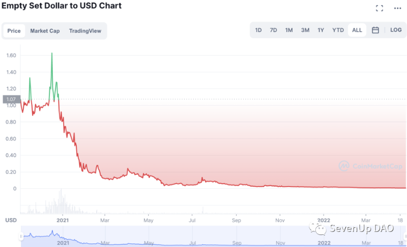
*Figure: ESD price chart*
BAC (Basis Cash) follows similar logic, differing only in details. Its system includes three tokens: BAC (stablecoin), BAS (staking receipt), and BAB (bond). When BAC trades below $1, users can buy BAB at a discount. When BAC trades above $1, BABs are redeemed first into BAC; leftover supply goes to BAS stakers.
Clearly, BAC fails to resolve the systemic deficit caused by excessive BAB issuance—and in fact maintained stability for an even shorter period than ESD.
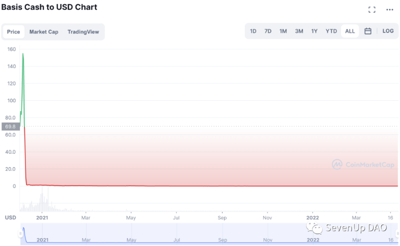
*Figure: BAC price chart*
**V. Next-Gen Algorithmic Stablecoins: Partial Collateral, Dual-Token Models, and Ponzi Schemes**
Next-generation algorithmic stablecoins adopted more sophisticated designs. Frax stands out as a representative success story. Yet, clever mechanics alone cannot prevent collapse—Iron Finance serves as a cautionary tale. Meanwhile, projects like OHM masquerade as “algorithmic stablecoins” but function as outright Ponzi schemes, fundamentally different in intent and trajectory.
**5.1 FRAX: Prudent Collateral Ratio, Deep Liquidity Pools**
FRAX (Frax Finance) operates with two tokens: FRAX, the $1-pegged stablecoin, and FXS, the governance token absorbing FRAX’s volatility and reflecting protocol growth.
The key concept is the Collateral Ratio (CR), determining how much USDC is needed to mint one FRAX. CR adjusts dynamically: starting at 100% (fully collateralized), it is recalibrated hourly based on FRAX’s price. If FRAX > $1, CR decreases by 0.25%; if < $1, it increases by 0.25%. Governance can modify parameters. The current CR is 86.75%.
> Example: At CR = 85%, minting 1 FRAX requires depositing 0.85 USDC and FXS worth $0.15. Conversely, redeeming 1 FRAX yields 0.85 USDC and $0.15 worth of FXS. This enables arbitrage when FRAX deviates from $1, stabilizing its price.
Critically, **this mechanism transfers FRAX’s volatility and sell pressure onto FXS.** To prevent FXS collapse, the team endowed it with value: staking FXS grants governance rights and 0.4% fees from minting/redeeming FRAX. Additionally, the AMO (Algorithmic Market Operations) reinvests collateral pool assets, sharing profits with FXS stakers.
After over a year, FRAX emerged as a winner in Curve’s “liquidity wars”: as of April 26, FRAX held 16.4% of CVX voting power, alongside Terra in the top tier.
This victory created deep liquidity pools—FRAX-3Crv (USDT, USDC, DAI) pool depth reached $2.8 billion, with $1.14 billion in the three major stablecoins. This implies destabilizing FRAX would require dumping over $1 billion. Moreover, deep liquidity strengthens FRAX’s position in DeFi, expanding use cases and earning potential.
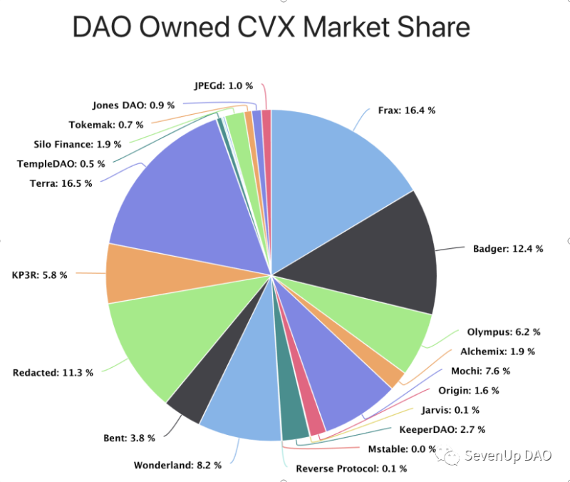
*Figure: CVX market share*
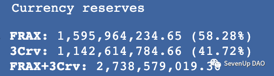
*Figure: FRAX-3Crv pool depth*
**FRAX is among the most stable algorithmic stablecoins and has endured significant stress tests.** Its anti-death-spiral strategy offers valuable lessons: high USDC collateralization (increasing when price dips) boosts confidence; deep liquidity pools with major stablecoins make short-term attacks impractical. Today, Frax Finance actively builds DeFi partnerships to sustain long-term competitiveness.
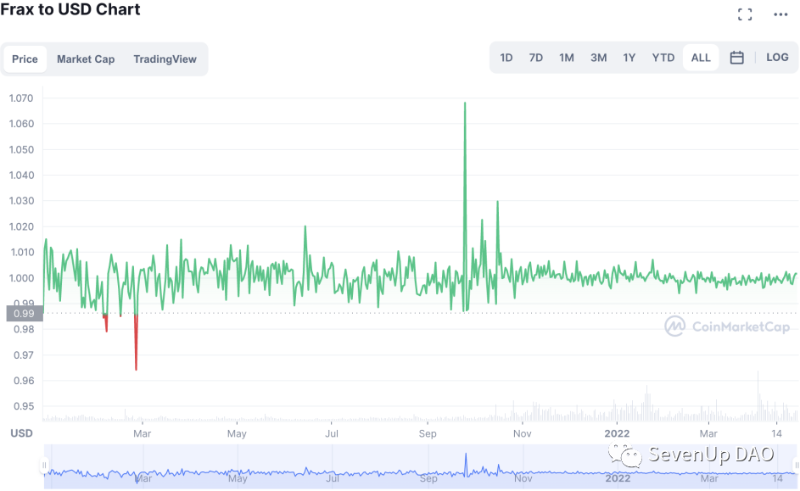
*Figure: FRAX price chart*
Some believed Frax’s dual-token model was central to its stability. While using a secondary token to absorb volatility is innovative, it doesn’t eliminate the fundamental under-collateralization risk. The failure of numerous Frax clones proves this—most notably Iron Finance, whose $2.3 billion TVL collapsed in a single afternoon.
**5.2 IRON: Flaws in Initial Design Leading to Collapse**
Iron Finance’s codebase originated from Frax, operating on Polygon. It featured two tokens: IRON (stablecoin) and TITAN (governance token). Key differences:
- IRON required fixed 75% USDC collateral (vs. Frax’s initial 100%), with the remaining 25% covered by TITAN;
- Early staking yields were extremely high: 1.5% daily for USDC-IRON LP, 4.5% daily for USDC-TITAN LP.
Such yields were clearly unsustainable, yet attracted massive early participation—TVL surged to $2.3 billion in just two weeks. It’s hard to imagine any project sustaining 4.5% daily returns on $2.3 billion.
When TITAN peaked at $60, early sell-offs began. Within hours, TITAN dropped to $30, and IRON fell below $1. Theoretically, IRON’s redemption mechanism should stabilize price: regardless of TITAN’s fluctuations, redemption always yields “$0.25 worth of TITAN,” allowing arbitrageurs to restore parity.
But a fatal flaw undermined this: the oracle used a “10-minute average price” for TITAN. **During rapid drops, this lagging price significantly exceeded the true market value, making users realize the redeemed TITAN was worth less than $0.25—breaking the arbitrage logic.** This destroyed confidence in IRON’s stability, triggering a stampede of IRON and TITAN sales—the “death spiral.”
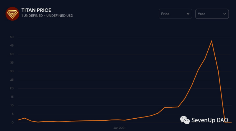
*Figure: TITAN price chart*
Iron’s collapse teaches several lessons:
1. The “death spiral” remains an ever-present threat—not avoidable by copying mechanisms.
2. High early yields attract users and visibility but amplify instability. Teams must assess their ability to sustain price support.
3. Even minor design flaws can determine a project’s fate.
It’s speculated Iron copied Frax’s 10-minute oracle without adapting to Polygon’s faster settlement speed—requiring tighter time windows.
**5.3 OHM: A Ponzi Scheme in “Algorithmic Stablecoin” Clothing**
OHM (Olympus DAO), launched in 2021, gained fame for its “DeFi 2.0” narrative, “(3,3)” meme, skyrocketing price, and numerous clones. Though initially marketed as an “algorithmic stablecoin” with a DAI-based redemption floor, OHM’s core mechanisms incentivized behavior contrary to price stability—effectively turning it into a large-scale Ponzi scheme.
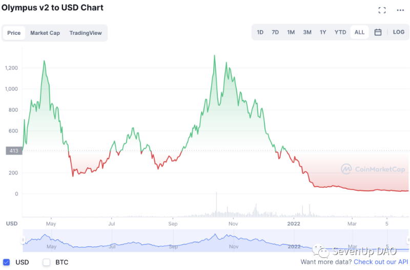
*Figure: OHM price chart*
Numerous analyses have detailed OHM’s innovations, so we won’t repeat them here. Briefly, the team used rebase + high staking yields, bonding to capture liquidity, and the “(3,3)” community meme to drive price upward—until inevitably spiraling downward. However, Olympus Pro, launched in early 2022, gave OHM some real DeFi utility, preventing complete collapse and maintaining a price above $20.
OHM exposed how the “algorithmic stablecoin” label can mask a Ponzi structure: if dual-token projects (like Iron) use unsustainable yields to inflate secondary tokens, why not skip the pretense? Drop the $1 peg, and let the main token soar directly via novel mechanics? But once OHM abandoned price anchoring, its long-term path diverged fundamentally from that of a “stablecoin.”
Indeed, many Ponzi schemes exploit the “algorithmic stablecoin” label. Even legitimate projects like FRAX and UST exhibit Ponzi-like traits in early stages. Hence, investing in algorithmic stablecoins carries extreme risk—participation demands utmost caution.
**VI. Chain-Specific Algorithmic Stablecoins: Nation-States and Fiat Analogies**
Recently, major blockchains have launched native stablecoins—becoming a key trend. Here we analyze UST’s design and trajectory, with brief commentary on others.
**6.1 UST: Burn-to-Expand, Attempting “Too Big to Fail”**
UST is issued by the Terra blockchain, forming a dual-token system with LUNA: users burn $1 worth of LUNA to mint 1 UST, or burn 1 UST to mint $1 worth of LUNA.
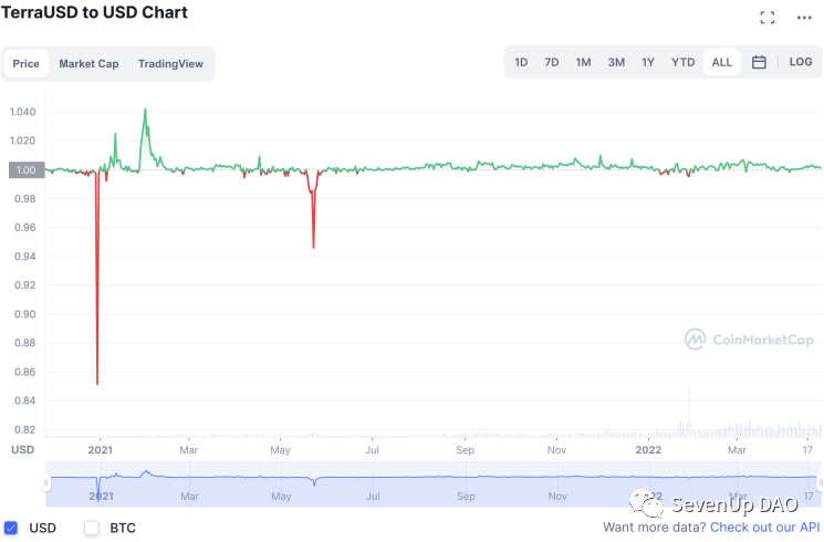
*Figure: UST price chart*
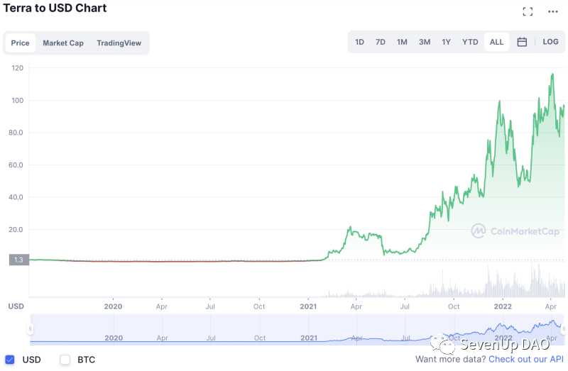
*Figure: LUNA price chart*
Mechanically, UST derives value from LUNA. But why hold UST? Because **Anchor Protocol on Terra offers 20% annual yield on UST deposits—paid in UST, not project tokens, eliminating exposure to token depreciation.** Compared to other stablecoin yields, 20% is exceptionally high. Given Anchor’s transparency, backing by Korean conglomerates and global capital, users migrated idle stablecoins to UST. Today, UST’s $18.3 billion market cap dwarfs FRAX’s $2.7 billion—even exceeding half of LUNA’s $33.4 billion valuation.
Anchor earns by lending deposited UST (borrowers must over-collateralize), and reinvests collateral. Yet analysis shows (see: “On the Rise of Algorithmic Stablecoins: Terra, Olympus, FRAX”) Anchor’s income falls short of interest payouts—resulting in an estimated $1.7 billion annual deficit, currently covered by LFG (Luna Foundation Guard).
Everyone knows **20% APY is unsustainable.** Left unchecked, reducing yields could trigger panic selling, causing LUNA’s price to spiral down and potentially collapse the entire system. Terra is taking two measures to avoid this:
- Purchasing hundreds of millions in BTC to eventually back UST—transforming UST into something akin to Bretton Woods-era USD: “Though not fully backed by BTC, we hold substantial reserves. As long as there’s no mass redemption rush, the system holds. And redeeming UST for BTC will incur high fees and friction.”
- Expanding UST’s DeFi integrations and liquidity depth—e.g., partnering with Frax to build a 4Crv pool on Curve, aiming to replace DAI as a foundational DeFi stablecoin; enabling UST minting on Avalanche. These moves aim to provide redemption buffers and create a “too big to fail” effect: if UST collapses, the entire DeFi ecosystem suffers.
This “too big to fail” dynamic already exists—exemplified by USDT. With nearly $83 billion market cap, few believe Tether holds full dollar reserves. Yet, due to USDT’s dominance and ubiquity, the market collectively overlooks its risks. A USDT collapse would be catastrophic—so everyone tolerates its flaws. Tether enjoys immense seigniorage benefits, and despite persistent accusations of manipulation, market impact remains limited. USDT’s “too big to fail” status and monetary privileges are widely observed.
Ultimately, every chain-specific algorithmic stablecoin aims to become a crypto-native “USDT”—a trusted credit currency. Long-term, for UST to solidify its role as a medium of exchange, payment method, or unit of account, ecosystem expansion is essential. Compared to non-chain-backed stablecoins like FRAX, UST enjoys inherent advantages in building real use cases. As previously stated, if top-tier apps exclusively use UST for interactions, users will naturally prefer holding UST—not for yield, but for convenience.
**6.2 USDN: Clear Manipulation, a Ponzi Vehicle**
In March 2022, Waves (“Russia’s Ethereum”) launched USDN, sending WAVES price from under $10 to over $50. USDN’s minting mechanism resembles UST’s, but its yield consists of a fixed rate multiplied by the market cap ratio of WAVES to USDN.
Theoretically balanced, this becomes a Ponzi enabler when WAVES price rises: buy WAVES → mint USDN → stake USDN to borrow USDC → use USDC to buy more WAVES—creating a self-reinforcing loop that ultimately extracts USDC from retail users using collapsing WAVES and USDN. On-chain analysis revealed coordinated price manipulation, with even Waves acknowledging it (though blaming third parties).
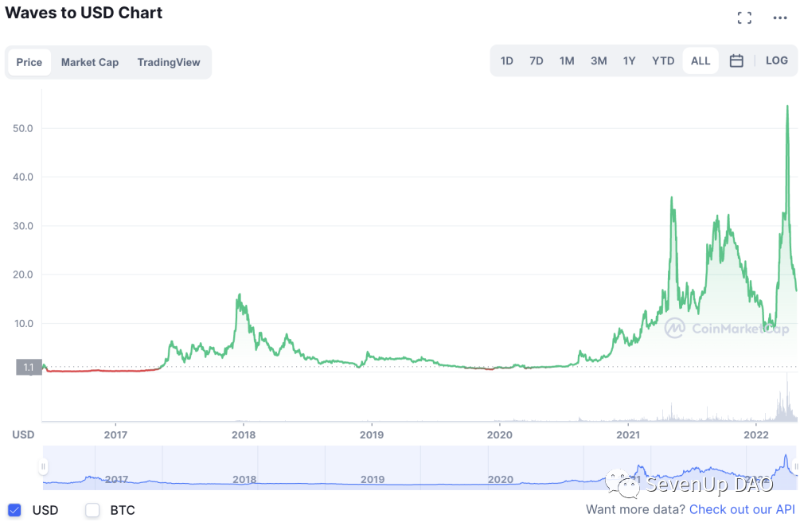
*Figure: WAVES price chart*
WAVES has since crashed, and USDN remains below $1. Clearly, USDN’s backers had no long-term vision—unlike UST’s subsidy-driven growth—treating it merely as a vehicle for a Ponzi scheme.
**6.3 NIRV: Short-Term User Acquisition, Long-Term Outlook Uncertain**
In April 2022, Solana launched Nirvana. Its design features innovations: dual-token model (NIRV stablecoin, ANA governance token); a slowly rising “floor price” for ANA, allowing users to sell ANA to the protocol at floor price when market price dips.
Users buy ANA with USDC and stake it, gaining:
1. Borrow up to floor-priced NIRV (face value $1 each);
2. Receive prANA vouchers to buy new ANA at “market price − floor price”;
3. Earn 300% APY in ANA-denominated staking rewards.
Compared to FRAX or UST, Nirvana resembles OHM: the floor price acts as a theoretical “backstop,” but like no one redeeming 1 OHM for 1 DAI, ANA’s market price far exceeds floor price—making entry costly and redemptions rare. Staking ANA allows borrowing NIRV, which can then be used to buy more ANA at a “discount,” combined with high yields, driving ANA’s price skyward—similar to OHM. At launch, it triggered massive FOMO, with the community dubbing it “left foot on right foot, spiraling to heaven.”
However, while mimicking OHM, Nirvana does include a functional stablecoin, NIRV. **Yet using NIRV as a medium of exchange faces efficiency issues due to low capital utilization.**
> Example: ANA trades at ~$16, floor price $5. So $16 USDC yields only 5 NIRV for ecosystem use—far less efficient than FRAX or UST.
In short, Nirvana effectively used OHM-style tactics for rapid user acquisition and price inflation. Long-term viability depends on whether ANA’s market price converges toward its floor and whether it can build meaningful Solana-based applications—areas warranting further observation.
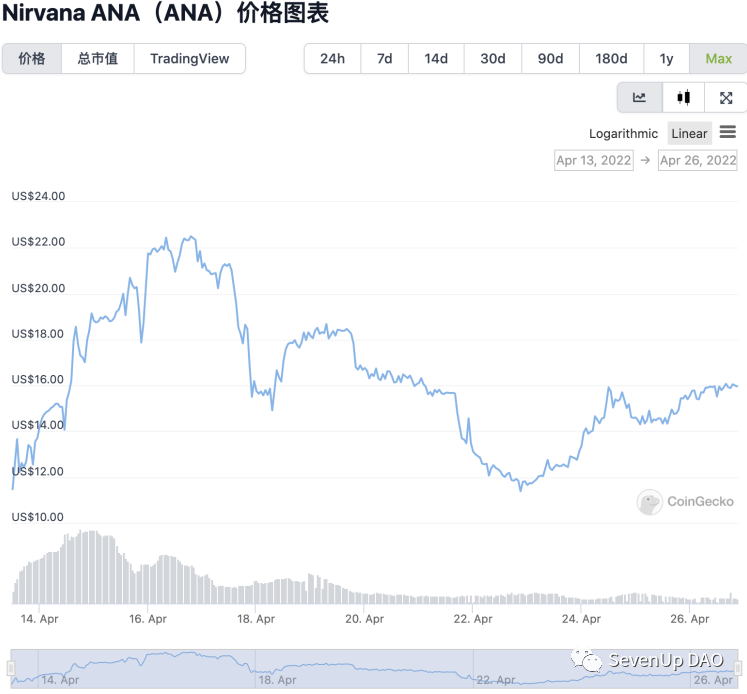
*Figure: ANA price chart*
**VII. Conclusion**
Through analysis of various algorithmic stablecoin projects, we can outline a developmental pathway:
- **Early stage:** Attract users through well-designed incentives and attractive staking yields;
- **Mid-term:** As the project scales, gradually phase out unsustainable yield components, deepen integration and liquidity pools with mainstream crypto assets to strengthen confidence and resist bank runs;
- **Long-term:** For algorithmic stablecoins to succeed, they must achieve a “too big to fail” status in the crypto world and develop extensive real applications, embedding their “$1 stability” into users’ subconscious.
For general investors, participating in algorithmic stablecoins carries extremely high risk—especially new projects, where prices can crash to zero overnight. Participation demands great caution. However, these projects often pioneer innovative tokenomics to maintain stability without real-world backing—innovations that may influence future crypto projects. Thus, studying this space remains highly valuable.
Join TechFlow official community to stay tuned
Telegram:https://t.me/TechFlowDaily
X (Twitter):https://x.com/TechFlowPost
X (Twitter) EN:https://x.com/BlockFlow_News
Add to Favorites
Share to Social Media