

Curve Stablecoin Design Whitepaper: Continuous Liquidation / No-Liquidation AMM
TechFlow Selected TechFlow Selected
Curve Stablecoin Design Whitepaper: Continuous Liquidation / No-Liquidation AMM
Hope the proposed mechanism can address the risks associated with liquidations for stablecoin and lending purposes.
Author: JamesX, iZUMi Research
This is a bilingual reference version of the Curve stablecoin design whitepaper, with added explanatory notes in Chinese and corrections to some spelling errors in the original. For reference and study purposes.
Overview
Several key concepts are central to this stablecoin design: the Lending-Liquidating AMM Algorithm (LLAMMA), PegKeeper (peg maintenance mechanism), and monetary policy. However, the core innovation lies in LLAMMA: replacing traditional over-collateralized loan liquidation processes with a specialized-purpose AMM.
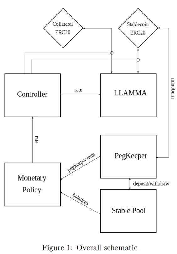
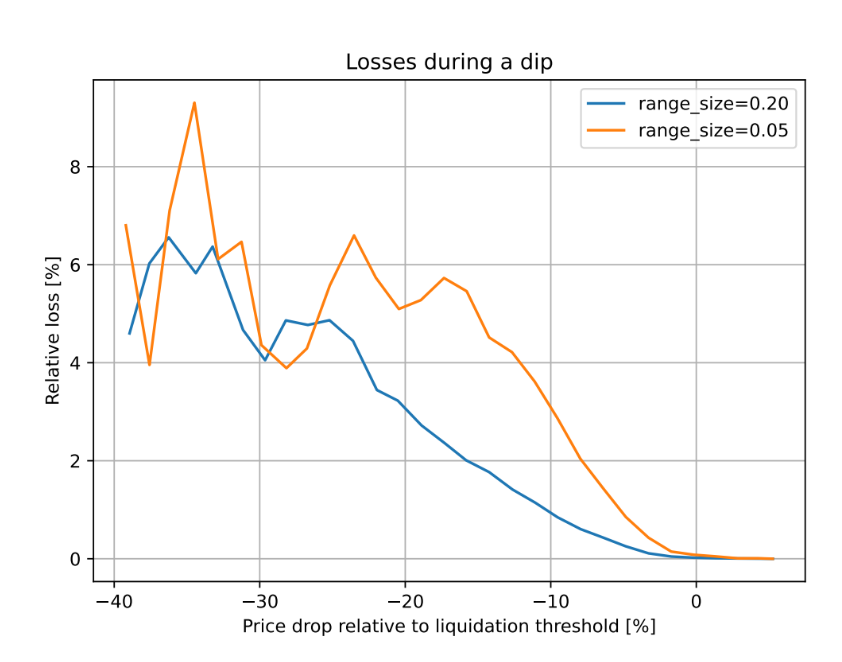
Figure 2: Dependence of losses on price movements relative to the liquidation threshold. Observation window is 3 days.
In this design, even if a user’s collateral experiences a price drop followed by a rebound—while remaining at or near the liquidation threshold—no significant loss occurs.
For example, simulations based on historical ETH/USD data since September 2017 show that if a CDP is left unattended for 3 days and the price drops 10% below the liquidation price during that period, only about 1% of the collateral is lost.
Continuous Liquidation / No-Liquidation AMM (LLAMMA)
The core idea behind the stablecoin design is the Lending-Liquidating AMM Algorithm (LLAMMA). The concept involves converting between collateral (e.g., ETH) and the stablecoin (here referred to as USD). When the collateral price is high, the user's deposit remains entirely in ETH; but as the price falls, it gradually converts into USD stablecoins. This differs significantly from traditional AMMs, where stablecoins like USD are placed on one side (top half of the curve) and volatile assets like ETH on the other (bottom half).
The following description does not constitute a fully self-consistent rigorous proof. Many aspects—especially the invariant—are derived heuristically from multiple considerations. A complete mathematical formulation may require further research, but the current description is considered sufficient for implementation in smart contracts.
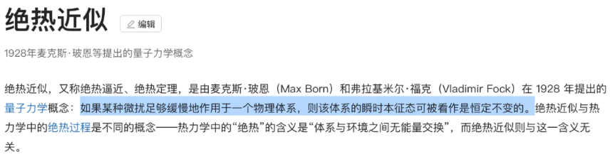
This mechanism can only function with an external price oracle. In brief, if one constructs a typical AMM (e.g., with a bonding curve shaped like a hyperbola) and shifts its "center price" from lower to higher values, tokens will adiabatically convert from USD to ETH (or vice versa), while providing two-way liquidity throughout the process (see Figure 3). This is conceptually similar to “avoided crossing” (also known as Landau-Zener transition) in quantum physics—though purely analogical, as the actual mathematical description may differ significantly.
The range over which liquidity is concentrated is called a “band.” Within a constant oracle price band, there is liquidity ranging from pcd to pcu. We seek functions pcd(po) and pcu(po) that grow faster than linearly with po—i.e., their growth rate exceeds that of po (see Figure 4). Additionally, define prices p↓ and p↑ such that p↓(po)=po and p↑(po)=po, representing the bottom and top ends of the band in the adiabatic limit (e.g., when p=po).
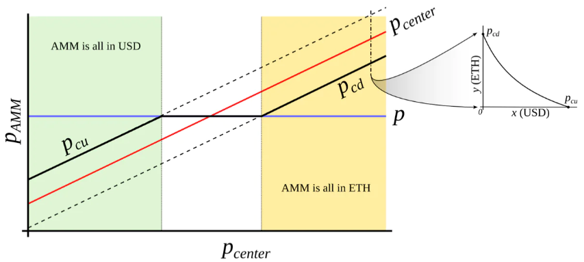
Figure 3: Behavior of an “AMM with external price source.” The external price pcenter determines the center around which liquidity is formed. The AMM supports concentrated liquidity between prices pcd and pcu, where pcd < pcenter < pcu. When the current price p moves outside the [pcd, pcu] range, the AMM becomes fully converted either into stablecoins (at pcu) or into collateral (at pcd). When pcd ≤ p ≤ pcu, the AMM price equals the current market price p.
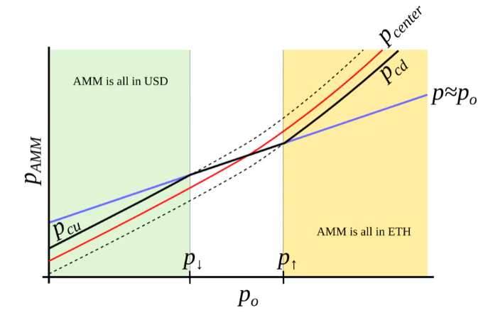
Figure 4: Desired AMM structure. We aim to construct an AMM where pcd and pcu are functions of po that grow super-linearly with po. In such a setup, when ETH is expensive, the AMM fully converts to ETH; when ETH is cheap, it fully converts to USD.
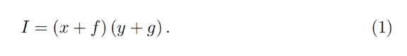
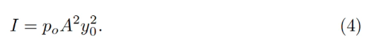
We begin similarly to Uniswap V3, using multiple bands with “virtual balances” preserving the hyperbolic shape of the bonding curve. Let x be the amount of USD and y the amount of ETH. Then the “enhanced” constant-product invariant becomes:
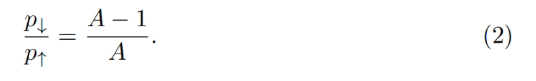
We can also write x₀ ≡ x + f and y₀ ≡ y + g so that the invariant takes the familiar form I = x₀y₀. However, f and g are not constant—they vary with changes in the external oracle price po (and so does the invariant I, meaning it's only invariant when po is fixed). At any given po, f and g remain constant across a single band. As defined earlier, let p↑ denote the upper price bound of the band and p↓ the lower. Our definition of A—a measure of liquidity concentration—is as follows:
The desired property we seek is: higher oracle prices po should result in higher internal prices for the same reserves, causing the current market price (on average tracking po) to fall below this level, thereby pushing trades toward full ETH exposure (and vice versa in the opposite direction). Many functional forms could satisfy this, but we need one satisfying:
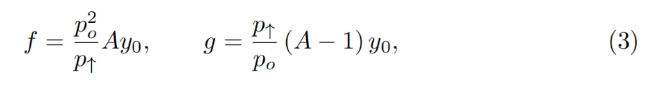
Here, y₀ is a quantity related to po indicating the current band’s deposit measured in ETH. It is defined such that when the current price p, p↑, and po all coincide, then y = y₀ and x = 0 (see the point at po = p↑ in Figure 4). Substituting y accordingly:
Since price equals dx₀/dy₀, for a constant product invariant this gives:
One can substitute x=0 or y=0 to verify consistency under conditions po=p↑ or po=p↓.
Typically, for a given band, we know p↑, hence p↓, po, constant A, and current deposits x and y. To compute everything else, we must determine y₀. This can be found by solving a quadratic equation derived from the invariant:
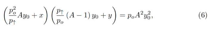
This leads to a quadratic equation in terms of y₀:
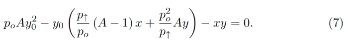
In the smart contract, this quadratic equation is solved within the get_y0 function.
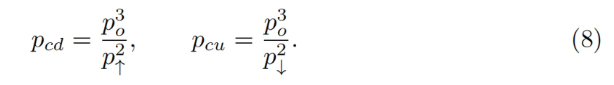
When the oracle price po remains constant, the AMM operates normally—selling ETH when price rises and buying ETH when price falls. By substituting x=0 into the invariant equation for the lower boundary price pcd, or y=0 for the upper boundary price pcu, we derive the AMM price under current values of po and p↑:
Another important practical question arises: if price changes slowly enough that the oracle price po can “adiabatically” follow the movement within a band, how much ETH (denoted y↑) would ultimately remain in the band if the price increases, or how much USD (x↓) if the price decreases—given initial x and y and starting from p=po? While not immediately solvable analytically, numerical computations yield a surprisingly simple answer:
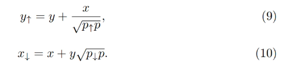
These results will be used in assessing lending safety and potential AMM losses.
Now we have a description for a single band. We divide the entire price space into contiguous bands, where the lower price p↓ of one band meets the upper price p↑ of the next. Setting a base price pbase and a band index n:
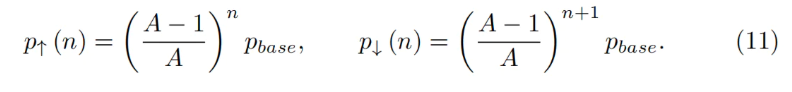
For any band, it can be shown that solutions to Equations 7 and 5 lead to:
This confirms that there are no gaps between adjacent bands.
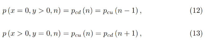
Trades preserve the invariant in Equation 1, yet when the oracle price po changes, the internal price within the AMM shifts: when po decreases, the internal price increases, and vice versa—with a cubic dependence evident from Equation 8.
LLAMMA vs Stablecoin
A stablecoin here functions as a CDP where users borrow stablecoins against volatile collateral (cryptocurrencies like ETH). The collateral is deposited into a price range (band) within LLAMMA. If the collateral price declines gradually, ETH is automatically converted into sufficient stablecoins to cover the loan repayment (via self-liquidation, external liquidation if collateral ratio approaches danger levels, or simply waiting for price recovery without closing).
When a user deposits collateral and borrows a stablecoin, the LLAMMA smart contract determines the corresponding band. As the collateral price fluctuates, conversion into stablecoins begins. When the system goes “underwater,” the user already holds enough USD to repay the debt. The available stablecoin amount can be calculated via a public get_x_down method. If this value approaches the liquidation threshold too closely, external liquidators may intervene (though typically unnecessary unless price stays low for days or weeks; never required if price recovers quickly). When far above “liquidation,” a healthy position returns the ratio of get_x_down to debt plus increased collateral value.
When interest is charged on the stablecoin, this must be reflected in the AMM. This is achieved by shifting all price grids upward proportionally to the interest rate r, implemented via a base price multiplier. Thus, as long as the interest rate is positive, the multiplier increases over time.
When computing get_x_down or get_y_up, we first determine the quantities x* and y* of stablecoin and collateral that would exist if the current price moved to the oracle price po. Then, we calculate how much stablecoin or collateral would result if po were to adiabatically shift to the lowest price in the lowest band or highest price in the highest band, respectively. This provides a robust metric for expected stablecoin proceeds, independent of transient market prices—an important defense against sandwich attacks.
Note that LLAMMA uses po defined as the ETH/USD price as its input. Our stablecoin may trade below (ps < 1) or above (ps > 1) its peg. If ps < 1, then the effective price within LLAMMA becomes p > po.
Under the adiabatic approximation, p = po / ps, meaning all collateral ↔ stablecoin conversions occur at a higher oracle price—as if the oracle price were lower and equal to:
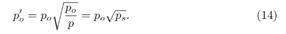
At this adjusted price, the quantity of stablecoins obtained upon conversion is scaled up by a factor of 1/ps (when ps < 1).
Persistently having ps > 1 is undesirable; hence we employ a stabilizer mechanism (discussed next).
Automatic Stabilizer and Monetary Policy
When ps > 1 (e.g., due to increased demand for the stablecoin), anchor reserves are created through asymmetric deposits into the stableswap Curve pool—between the stablecoin and redeemable reference coins or LP tokens. Once ps > 1, the PegKeeper contract is permitted to mint uncollateralized stablecoins and deposit them unilaterally into the stableswap pool, ensuring the final price does not fall below 1. Conversely, when ps < 1, PegKeeper may withdraw (asymmetrically) and burn stablecoins.
These actions cause rapid depreciation when ps > 1 and appreciation when ps < 1, because asymmetric deposits and withdrawals shift the price. Even though this portion of “minting” is uncollateralized, the stablecoin appears implicitly backed by liquidity in the stableswap pool. Overall, the minting/burning cycle proves profitable while enhancing stability.
Let dst represent the quantity of stablecoins minted by the stabilizer (debt), and fdx() be the function calculating the redeemable USD needed to buy stablecoins via the stableswap AMM’s get_dx. To prevent the “reserve” from growing excessively large, we implement a “slow” stabilization mechanism by adjusting the borrowing rate r:
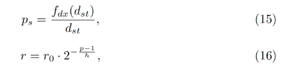
where h is the change in ps, and r adjusts twice as fast (higher ps leads to lower r). The stabilizer debt dst will balance at different levels depending on how far ps deviates from 1. Therefore, instead of manual tuning, we can reduce r₀ when dst/supply exceeds a target threshold (e.g., 5%), incentivizing borrowers to take loans and sell stablecoins (lowering price and forcing system to burn dst). Conversely, increase r₀ when dst/supply is low, encouraging loan repayments and pushing ps upward (forcing system to accumulate more dst and stabilizer deposits).
Conclusion
We hope the proposed mechanism effectively mitigates the risks associated with liquidations in stablecoin and lending systems.
Furthermore, the stabilizer and automatic monetary policy mechanisms can help maintain price peg stability without requiring an oversized PSM (Peg Stability Module).
Join TechFlow official community to stay tuned
Telegram:https://t.me/TechFlowDaily
X (Twitter):https://x.com/TechFlowPost
X (Twitter) EN:https://x.com/BlockFlow_News