
The Inheritance and Innovation of AMM Model Design in NFT Transactions
TechFlow Selected TechFlow Selected
The Inheritance and Innovation of AMM Model Design in NFT Transactions
How to design a DEX from scratch?
Article: @Buidler DAO
Author: @Joseph Xu
Author's Note
Over the past one or two years, AMM model algorithms that have been proven effective by the market have rarely undergone updates or iterations. The core issue of AMMs has gradually shifted from designing efficient and rational algorithms back to the essence of financial markets—liquidity. Today’s NFT assets face similar challenges regarding liquidity scarcity. Yet, the NFT market still lacks an effective DEX capable of truly solving issues like trade matching and price discovery from the perspective of liquidity aggregation. Today, starting from AMM DEXs, we’ll share how we drew inspiration and insights from existing AMM designs when building Midaswap Protocol, our NFT liquidity protocol, and how we innovated upon these established models to address unique pain points and demands in the NFT market.
— Joseph
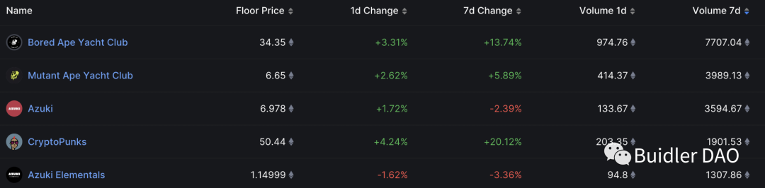
Since Q3, the NFT market has experienced significant volatility, with blue-chip NFTs plummeting. Setting aside influences from project teams and issuers, liquidity remains the most critical issue in the NFT market. Currently, on EVM chains, we can roughly define NFTs as derivatives of ETH.
Moreover, whether or not you've participated in NFT trading, you’ve likely noticed the rapid success of blur.io. In terms of liquidity solutions, Blur seems to have delivered a high-scoring solution from a centralized exchange/aggregator perspective. It now holds nearly the largest share of bid-side liquidity in this market. As a latecomer, especially given OpenSea's long-standing dominance, its rapid rise is remarkable. We could say Blur has executed centralized liquidity solutions exceptionally well. However, for dApp developers and public chain ecosystems, we believe centralization may only be part of the trading landscape. We seek ways to build our own on-chain NFT exchanges—or NFT DEXs. Therefore, today we aim to explore the following questions:
-
What liquidity model should be adopted when building a decentralized NFT exchange?
-
When designing a decentralized NFT AMM, what aspects of existing DEX AMM models are worth learning from?
-
Given that ERC721 and ERC20 represent fundamentally different asset types, how should their AMM models differ in design?
We’ll approach these questions together today, sharing both exploration and insights, while walking through the thought process behind our product, Midaswap, during its model design phase.
How to Design a DEX from Scratch
Let’s begin with a more abstract question: when designing a DEX, what conceptual struggles must we navigate, or what key decisions must we make?
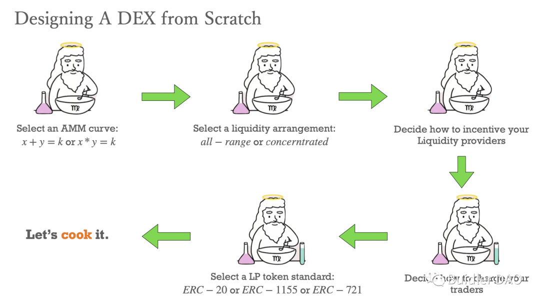
First, most people know that choosing an AMM curve is likely the first directional decision every AMM designer must make. Indeed, x+y=k, x·y=k, or even Balancer’s more customized multi-token pool invariant functions—all fall under CFMM (Constant Function Market Makers). Here, x and y, along with b in Balancer’s formula, represent the asset balances or supply within a given market or liquidity pool. These models re-price assets based on proportional or other constructed quantitative relationships between supplies. Thus, the choice of curve often reflects the type of target assets the liquidity protocol aims to attract. For stablecoin trading, Curve V2 uses a hybrid invariant function: near equilibrium, it behaves more like a constant sum curve; farther away, it resembles Uniswap v3’s constant product model. Hence, there is no perfect AMM curve—only one best suited to your specific market.
The second challenge concerns how liquidity should be distributed. This involves two aspects: whether liquidity spans the entire price range, a fixed interval, or a user-defined price range. This distinction separates Uni V2 from Uni V3. Uni V2 employs a simple model, distributing both tokens across the full range while strictly adhering to xy=k. However, this leads to low capital efficiency at the curve’s extremes. Uni V3 introduced innovation by allowing LPs to provide liquidity within custom price ranges—Uni V3’s "range order" feature. Its AMM curve isn’t simply xy=k, but rather a superposition of countless such curves. Choosing a liquidity distribution method also raises another question: should liquidity be arranged horizontally or vertically? We’ll clarify this difference later, as it may not yet be intuitively clear.
The third and most important question is how to incentivize LPs. LPs are the most crucial participants in any DEX or game-like system. Without LPs, there is no liquidity depth and thus no good trading experience. Every DEX faces the same dilemma: how to attract LPs? All DEXs use trading fee revenue to attract LPs. Some newer protocols create additional composability benefits—for example, staking LP tokens or leveraging them in DeFi strategies. Projects like Paraspace allow Uniswap LPs to gain leveraged exposure through lending. These enhancements increase the appeal of liquidity pools. As previously noted, LPs are the essential element that keeps the liquidity flywheel spinning. Without strong mechanisms to attract LPs, the system cannot sustain positive momentum.
Fourth comes how to charge traders. Existing DEXs are fairly consistent here—the fee rate is typically set by the liquidity pool creator. Uniswap and Joe, for instance, offer multiple fee tiers. Notably, Joe V2 introduced dynamic fees, a feature Uni V4 later adopted via hooks. Dynamic fee rates represent a more advanced product design, as they can create a negative feedback loop to stabilize markets and, to some extent, hedge LPs against impermanent loss. While we won’t delve deeply into this topic here, it remains a critical consideration for any AMM designer.
Lastly, we must choose the form of LP tokens. There are many schools of thought here. Uni V2 uses ERC20, Uni V3 uses ERC721, and Joe V2 opts for ERC1155. In fact, the choice of LP token is jointly determined by the prior four decisions. The method of liquidity distribution and how liquidity is quantified within the protocol ultimately dictates the form of the LP token. Take Uni V2 vs. Uni V3: Uni V2 distributes liquidity across the full range, so any two LPs contributing the same proportion of total assets are considered equivalent. Hence, LP tokens within a Uniswap V2 pool are fungible—each contributes capital fairly at every price point. But Uni V3 introduced range orders (limit liquidity), redefining liquidity effectiveness. Not all liquidity participates in trades at all times—only liquidity within the current price range actively contributes capital to the market. Therefore, each LP’s position must be uniquely encapsulated using non-fungible tokens (ERC721), which appears to be the optimal solution so far. We don’t yet know what Uni V4 will do, but unless its liquidity model diverges significantly from V3, ERC721 will likely remain the best choice for LP tokens.
After navigating these five critical decisions, we establish the fundamental direction of an AMM protocol. This mental exercise helps structure our thinking. Only once these five areas are resolved do we truly step into the realm of detailed AMM model design, where finer-grained discussions become possible.
The Difficult Triangle of NFT AMMs
So far, we’ve discussed ERC20-based AMM DEX designs—including Uniswap, Curve, and Balancer, the dominant models in today’s market. Our focus today, however, is NFT AMMs. In an NFT AMM, one side of the trading pair consists of ERC721 NFTs, while the other holds fungible tokens like ERC20 or ETH. Placing these two fundamentally different asset types into a single AMM liquidity pool creates several inherent contradictions.
First and foremost, traditional NFT markets rely on a bid-ask model, resembling an order book. In an order book system, transaction speed deteriorates sharply when one side lacks liquidity. Consequently, NFT markets suffer from poor market-making tools and insufficient buyer-side liquidity. It's widely criticized that NFTs lack intrinsic value, and buyer-side liquidity is extremely scarce across all public chains. This severely limits turnover, inevitably leading to liquidity droughts. So, if we directly introduce NFT AMMs into the current DEX landscape without modification, we risk facing severe shortages of liquidity on the ETH or ERC20 side—an immediate challenge.
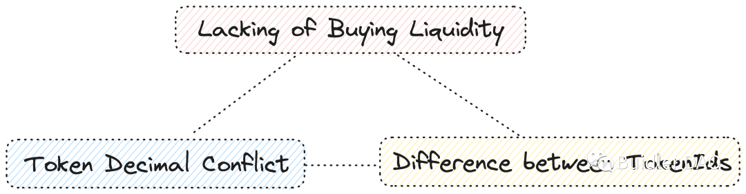
Second, a very practical issue: NFTs are traded whole. Due to their non-fungible nature, no NFT holder would willingly sell 10% of an NFT under normal circumstances. This contradicts the very nature of the asset. This introduces a problem: traditional AMM DEXs operate with infinitely divisible tokens. If mainstream ERC20s have 18 decimal precision, they can be subdivided down to that level, enabling prices to form a near-continuous curve. But NFT liquidity is inherently discrete, creating significant liquidity gaps. What kind of curve can bridge these gaps between discrete points? That’s a crucial question.
From another angle, because Token IDs are traded as whole units, NFT trading thresholds have historically been too high. When buying ETH, a retail user without enough USDT to buy one full ETH can purchase a fraction—say, $100 worth. But when an NFT is priced at 1 ETH, users cannot spend $100 to buy a fractional portion. Some protocols have proposed introducing fragmentation to NFTs. Fragmentation is a straightforward solution, but it introduces the third leg of the difficult triangle: do fragmented NFTs retain the original NFT’s tradable properties?
When an NFT collection is issued, metadata attributes determine the rarity of individual or groups of NFTs. Different rarities lead holders to have varying price expectations. But fragmentation treats all NFTs deposited into a fragmented liquidity pool equally—we cannot distinguish which fragments originated from a high-rarity NFT within a fragmented pool.
These three issues constitute the core pain points any decentralized NFT protocol must confront. Without making thoughtful trade-offs among them, designing an effective NFT AMM will be extremely challenging.
Existing Solutions in the NFT AMM Market
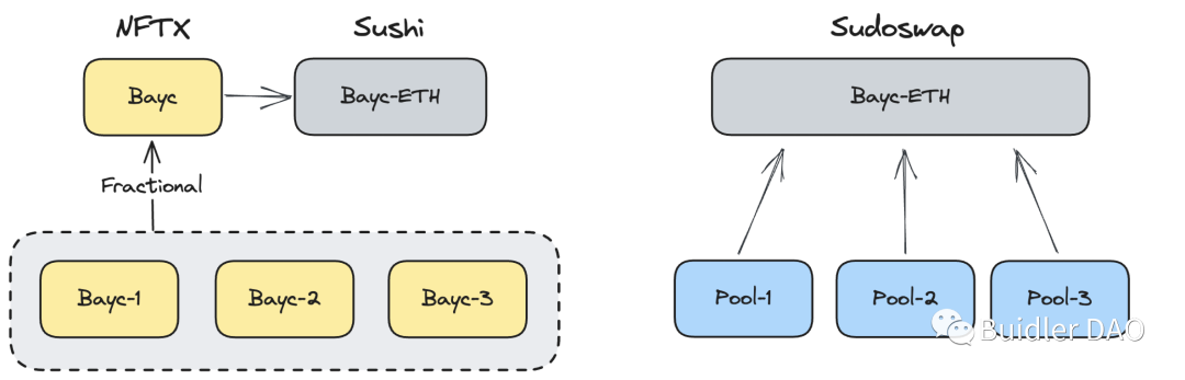
Now let’s examine mature solutions already present in the NFT AMM market. NFTX, for example, indiscriminately fragments NFTs into ERC20 tokens and builds trading pairs via SushiSwap pools. It crudely bypasses the token decimal conflict issue but ignores traders’ and holders’ differentiated perceptions of NFT rarity and pricing expectations. High-rarity NFTs cannot achieve proper value discovery under this AMM model.
Another project, Sudoswap, was the first native NFT AMM-like DEX. Why “AMM-like”? Because its role definitions differ somewhat from conventional AMMs. Let’s briefly explain Sudoswap: it turns each liquidity provider into a counterparty for traders. LPs design their own liquidity schemes using customizable bonding curves. Each LP owns their own liquidity pool and decides whether it’s a two-way or one-way pool. A two-way pool allows both buying and selling of NFTs—liquidity is bilateral, accepting swaps on either side. A one-way pool might hold only ETH, functioning like an NFT bid order; traders can sell NFTs into this pure ETH pool. Conversely, an NFT-only pool acts like a sell order.
In this setup, the LP role is diminished—LPs resemble traders with enhanced, customizable trading capabilities. But this creates two problems. First, if each LP operates their own liquidity pool, liquidity cannot be aggregated across pools. As previously noted, the biggest issue in NFT markets is the lack of buyer-side liquidity. Under this premise, fragmenting all liquidity into individual LP pools effectively siloes liquidity. This contradicts the fundamental purpose of AMMs: to aggregate liquidity within a market, deepen liquidity, and discover prices reflecting true market sentiment. Sudoswap fails here—each pool is isolated and does not influence others. Second, within a single pool, all NFTs are treated as having equal rarity. An LP adding three NFTs to their pool doesn’t individually price them. If an LP holds three NFTs of differing rarities and price expectations, they’d need to create three separate pools to reflect those differences.
Thus, while these two projects represent relatively mature offerings in the NFT AMM space, each resolves only part of the three core issues, making trade-offs that selectively ignore or compromise on others. So we ask: is there an NFT model that can better resolve these issues—or at least bring them to an acceptable balance?
Bonding Curves
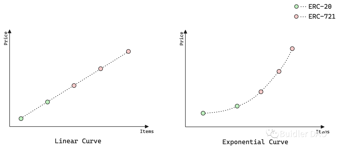
Next, we’ll explain Bonding Curves in detail, laying the groundwork for discussing deeper solutions. Bonding Curves are essentially mathematical functions designed to enable price discovery. They map asset supply to asset price. In the two charts above, the left shows a linear Bonding Curve, the right an exponential one. Green dots represent ERC20 positions in the pool, red dots represent ERC721s. Taking the left chart as an example: how is liquidity distributed in such a pool? At the lowest price—the starting point and next tick—liquidity is provided in FTs (ERC20). The top three ticks hold ERC721 liquidity. When a trader buys an NFT, the middle red dot becomes green. Each NFT purchase increases the price by a fixed amount; each sale decreases the index price by a fixed amount. The same applies to the exponential curve, except the fixed difference becomes a fixed ratio.
Sudoswap deserves credit for pioneering the use of Bonding Curves in NFT trading, giving LPs strong flexibility in market making. However, as mentioned, its design isolates liquidity across LP pools, causing its Bonding Curve to lose descriptive power over the broader market. We can’t infer overall market activity from a single pool. Its index price fails to reflect the characteristics of the entire NFT collection, falling into a “partial view” trap.
Inspiration from Existing DEXs
Considering the above pain points and existing product designs, we asked: what kind of NFT AMM could solve these issues? We began by studying mainstream ERC20 DEXs for inspiration.
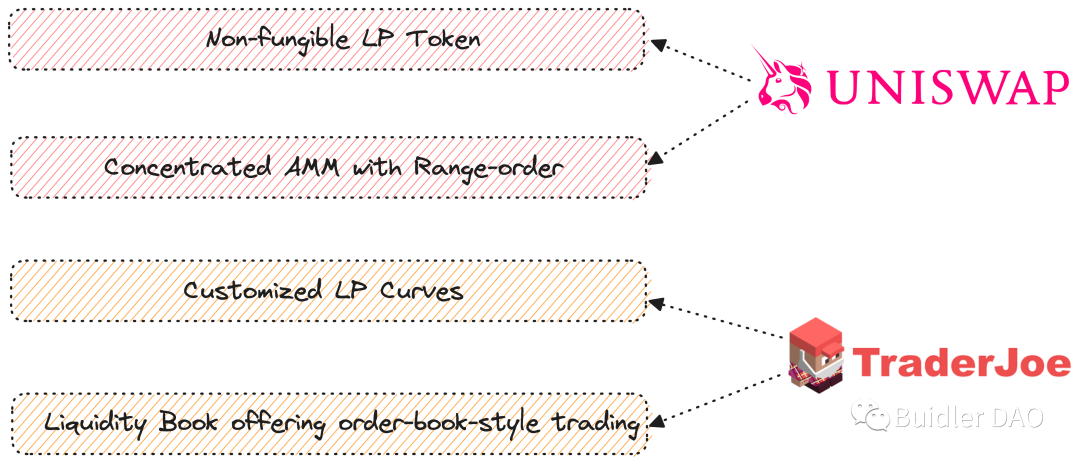
We closely examined Uniswap V3, which offered valuable inspiration. First, LPs can provide liquidity within defined price ranges—a concept similar to Sudoswap’s LP-defined bonding curves. This led us to wonder: could LPs freely place liquidity along a bonding curve within a shared pool? To support this, we’d likely need Non-Fungible LP Tokens—ERC721-based LP receipts—to clearly identify each LP’s unique, non-fungible position.
We also studied Joe V2’s protocol design, an upgrade over Uni V3. Joe V2 allows LPs to customize their curve shape and control liquidity sparsity. LPs can choose whether to spread liquidity evenly across their range or concentrate it at discrete points. Additionally, its Liquidity Book design enables order-book-like trading behavior at a micro level on-chain—a more modern approach to liquidity distribution.
From these two ERC20 DEXs, we derived four key insights. If ERC20 DEXs offer any guidance for NFT AMM design, it’s this: we must not ignore the intrinsic differences between NFT Token IDs—we should allow LPs to express differentiated price expectations for their assets. At the same time, we must not fragment liquidity into isolated private pools per LP—we should aggregate buy-side liquidity. Only aggregated liquidity delivers better trading experiences, lower slippage, and faster execution. Without aggregation, the experience of selling an NFT remains poor.
Design Philosophy of Midaswap AMM
With this background, we can now revisit how to design our own NFT AMM. Before that, consider a slightly tangential concept: if you’ve read about Uniswap V3, you know it uses a unique pricing unit called a Tick. A Tick is based on an exponential function of 1.0001—each increment multiplies the price by 1.0001. Thus, Ticks and prices are bijectively mapped. Why this design? All DEXs use a pricing scale to extract a finite, meaningful price grid from an otherwise infinite price space. Liquidity between these predefined ticks is ignored; we only deploy liquidity at designated Tick levels.
Another popular design is the Liquidity Bin. As the name suggests, Bins are like containers. We can think of liquidity at each price level as the height of a stack of contributions from LPs. For example, if I, as an LP, provide 1,000 USDC at the price of 1 ETH = 1,000 USDC, I raise the liquidity depth of that Bin by 1,000. If another LP adds 2,000, the depth becomes 3,000.
Why discuss this? Ticks align well with Uni V3’s incentive structure. But we believe Bins—vertical stacks of liquidity—are better suited for discrete NFT liquidity. We can treat each NFT liquidity unit as a small box stacked atop a Bin. Whenever an NFT holder or LP provides liquidity at a certain price, we visualize it as placing a box on that price-level Bin.
Why can't we simply copy an existing ERC20 DEX to solve all three problems? Because different NFT Token IDs have inherent rarity differences, leading to divergent value expectations—an intrinsic trait of NFTs. This contrasts sharply with most ERC20 DEXs, where at any moment, all trades in a pool occur at a single price. Therefore, if we aim to build a composite NFT market, we must combine the order-matching logic of centralized exchanges with the liquidity aggregation methods of DEX AMMs.
This led us to a new design: reintroducing the concepts of Best Offer and Floor Price—hallmarks of centralized NFT markets. Best Offer refers to the highest current bid for an NFT in the market—the buyer’s ideal price for a Collection. Floor Price is the lowest active sell order. With these two prices, we establish a liquidity market divide:

-
Above the Floor Price, we employ Bonding Curves to deliver an order-book-like trading experience for NFT traders. For example, if an LP chooses to provide NFT liquidity between 3 and 5 ETH, those NFTs are distributed across that price range according to their custom Bonding Curve. At any time, traders can select their desired NFT for trade. Each NFT is effectively price-locked by the LP. Each transaction causes a price adjustment along that LP’s Bonding Curve.
-
The AMM model operates at and below the Best Offer price. Here, FT liquidity providers act like buyers on Blur—offering bid-side liquidity. Their liquidity is fungible and aggregated at specified price points. By pooling this liquidity, we dramatically improve capital efficiency and trading performance, especially for users selling NFTs.
This NFT market design strikes a balance among the three pain points discussed earlier. We’ve found a reasonably balanced solution that maintains strong liquidity depth and low trading slippage without ignoring the uniqueness of individual NFT Token IDs. From the perspective of preserving native NFT trading needs, this may be the best approach we can envision today. Another key point: Best Offer and Floor Price are vital pricing indicators in NFT markets. Our design can serve as an on-chain Oracle, providing robust price discovery for NFT markets—eliminating reliance on external platforms for valuation. Furthermore, a fully on-chain NFT marketplace unlocks vast composability opportunities in DeFi. For instance, our LP tokens could be used as collateral for leveraged lending, and our Oracle could feed data into on-chain price feeds. These are precisely why we urgently need an efficient NFT AMM that meets the needs of both traders and LPs.
Join TechFlow official community to stay tuned
Telegram:https://t.me/TechFlowDaily
X (Twitter):https://x.com/TechFlowPost
X (Twitter) EN:https://x.com/BlockFlow_News