

Solana Players Must Know: JLP APY Prediction Principles and Interest Rate Trading Arbitrage Models
TechFlow Selected TechFlow Selected
Solana Players Must Know: JLP APY Prediction Principles and Interest Rate Trading Arbitrage Models
What is the leveraged interest rate trading protocol RateX? How to effectively use RateX to amplify returns?
Written by: @seanhu001, Founder of RateX.

TLDR: This article covers four key areas
1. Understanding the nature and stability of JLP: The article explains the mechanics of JLP and why it delivers stable high returns.
2. Analyzing and forecasting JLP APY: By breaking down the components of JLP APY (such as revenue sources and TVL), readers will understand the factors affecting APY and gain guidance on predicting both short-term and long-term APY trends.
3. JLP yield trading strategies: The article introduces various trading strategies, including leveraged yield speculation, fixed-income investments, and arbitrage opportunities based on APY, offering practical insights into yield trading.
4. Learn about RateX, the industry’s first leveraged interest rate trading protocol, and how to effectively use RateX to amplify returns.
Since the beginning of this year, JLP has emerged as one of the most closely watched asset types within the Solana ecosystem. It offers not only high yields but also remarkable value stability, making it a top choice for many investors during the current crypto bear market due to its superior risk-return profile. This article aims to help readers understand the core mechanics of JLP and demonstrate how to profit by analyzing and forecasting JLP's APY.
1. What is JLP?
JLP is Jupiter Perp's liquidity pool. The assets in the pool consist of SOL, WBTC, ETH, USDC, and USDT. The latest composition is shown below.
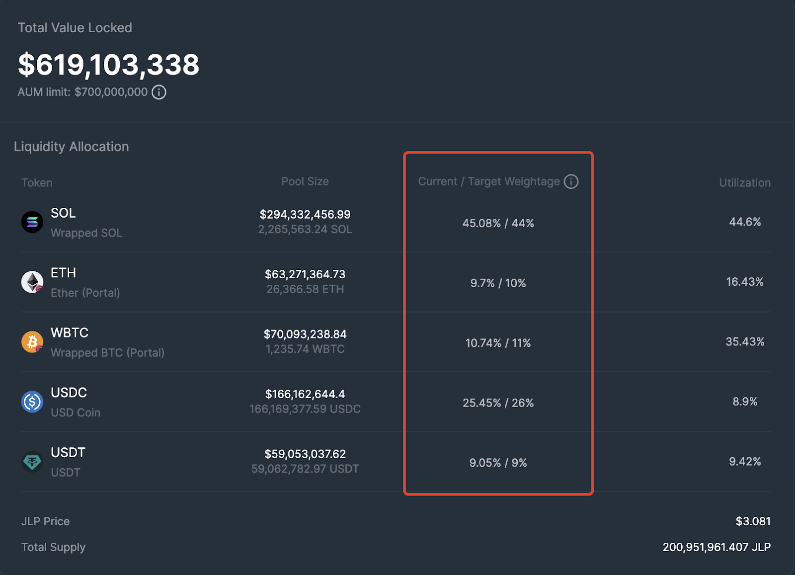
Target Weightage is set by the JUP team and adjusted via swap fees or mint/redeem fees. Current Weightage reflects the actual asset distribution in the pool. As seen, SOL holds the largest share at 45%, while ETH and WBTC each account for nearly 10%. The remaining 25% and 9% are allocated to USDC and USDT, respectively.
How should we understand the essence of JLP? Fundamentally, JLP is a combined pool of USD-denominated and crypto-denominated loans. We can divide the JLP Pool into two parts: the crypto portion and the stablecoin portion.
For the crypto portion—comprising SOL, ETH, and BTC—these assets are lent out to traders taking long positions. Traders borrow these assets and repay an amount equivalent in USD value at the time of borrowing. Thus, every new long position in crypto increases the dollar-denominated loan exposure within the JLP. When the utilization rate of a specific crypto such as SOL reaches 100%, it means all SOL in the JLP has effectively been converted into USD loans.
For the stablecoin portion—supporting two USD-pegged stablecoins, USDC and USDT—these assets are lent to traders opening short positions. Traders borrow dollars and must repay an equivalent quantity of crypto at the borrowed USD value. Hence, each new short position converts part of the stablecoins in JLP into crypto-denominated loans.
Therefore, we can derive a simple formula to calculate the true stablecoin ratio in JLP:
True Stablecoin Ratio = True Stablecoin Amount / TVL =
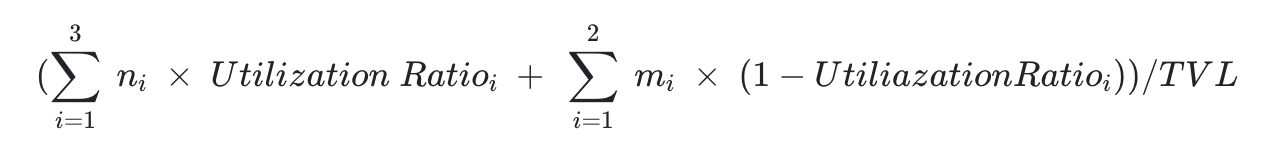
N represents the three crypto assets, and m represents the two stablecoins.
This formula clearly shows that when crypto utilization is high (many long positions) and stablecoin utilization is low (few short positions), JLP behaves more like a stablecoin pool. This implies that during bull markets, with heavy leveraged long activity, JLP becomes more stable in value. Of course, JLP may experience some impermanent loss (i.e., its pool value lags behind the sum of its underlying holdings during rallies, albeit with greater stability).
Conversely, when crypto utilization is low (few longs) and stablecoin utilization is high (more shorts), JLP starts to resemble a crypto-only portfolio. In bear markets, if long positions decrease while short positions increase, JLP’s value becomes more correlated with a crypto basket.
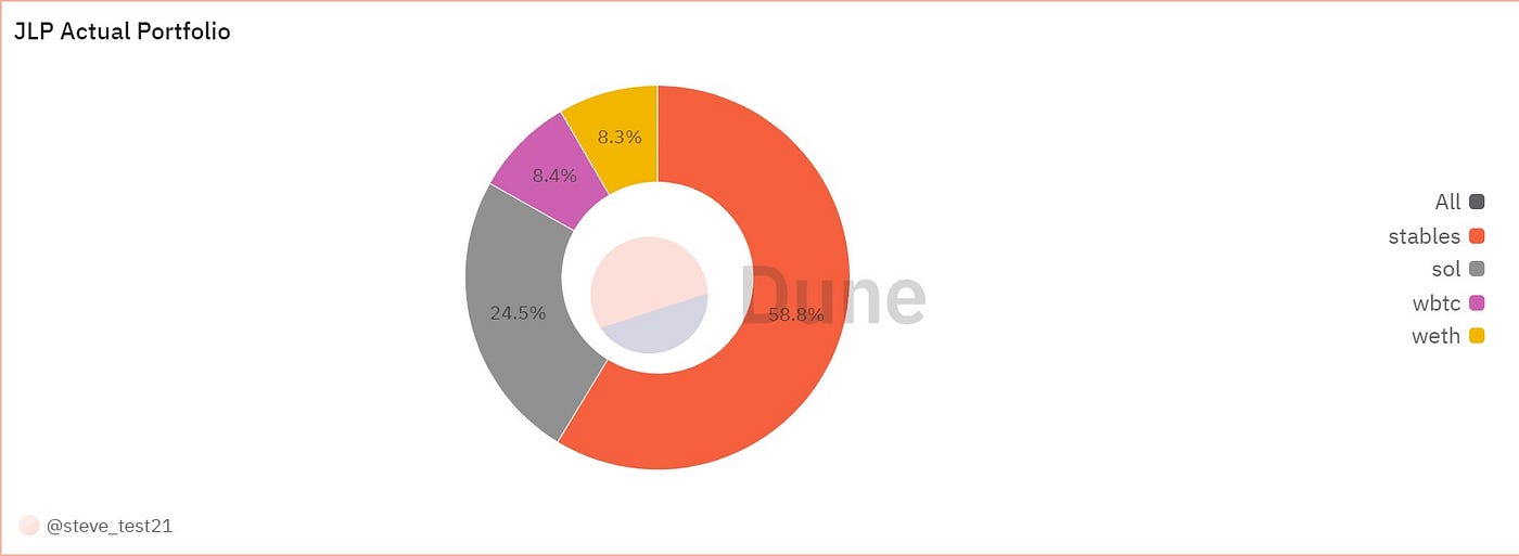
However, reality often deviates from this theoretical model. During bear markets, we observe that long positions on Jupiter Perp still dominate shorts. At the time of writing (September 5), the long-to-short ratio remains as high as 90%.
We can easily obtain current base data for the JLP Pool. According to our analysis, the current true stablecoin ratio stands at 58.8%. This is the primary reason behind JLP’s remarkable stability—when over half the portfolio consists of stablecoins, its value naturally resists volatility.
2. How to Predict JLP's APY
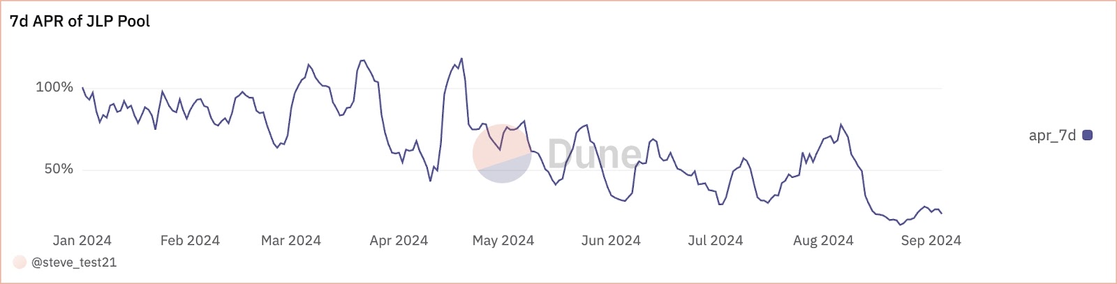
Let’s now examine another interesting aspect: JLP’s yield data, reflected in its weekly reported APY. Although JLP accrues yield directly into its net asset value, blending returns with price fluctuations of the underlying assets, we can still analyze on-chain or official APY data to isolate and study the yield component separately.
While Jupiter does not provide historical time-series APY data, we’ve constructed a 7-day average APY curve using on-chain data. The chart shows that JLP consistently delivers high returns, albeit with noticeable volatility. Despite a gradual downward trend as JLP scales up and market conditions turn bearish, APY remains around 30%.
Next, we’ll break down the components of JLP’s yield and guide you on forecasting both short-term and long-term APY trends.
First, the formula for JLP’s APY is straightforward:
APY = Earned Fees / TVL. This section will focus on analyzing both earned fees and TVL.
1. Composition of JLP’s Revenue Sources
According to Jupiter’s official documentation, JLP generates income through several mechanisms:
Opening and Closing Fees of Positions (consisting of flat and variable price impact fees)
Borrowing Fees of Positions
Trading Fees of the Pool, for spot assets
Minting and Burning of JLP
75% of the fees generated by JLP go back into the pool.
Thanks to Jupiter, we can view detailed breakdowns of these revenue streams on-chain (see here).
These daily figures form the foundation for forecasting JLP yields.
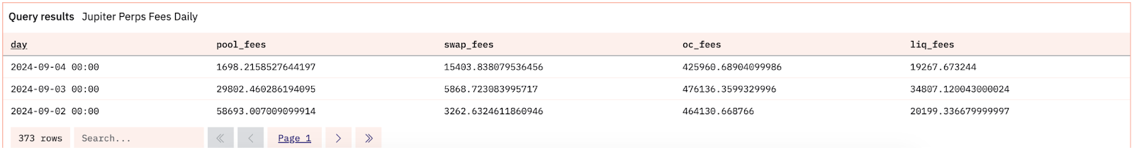
Here, pool_fees correspond to borrowing fees, swap_fees to trading fees, oc_fees to opening and closing fees, and liq_fees to liquidation fees.
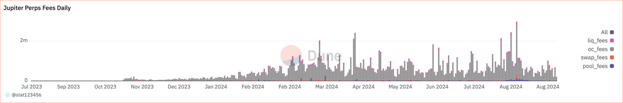
The chart above shows the time series of Jupiter Perps Fees since July 2023. We observe that oc_fees dominate overwhelmingly, so we primarily focus on them.
As per Jupiter’s documentation, opening and closing fees are calculated by multiplying transaction volume by a fee rate of 0.06%. While this rate is dynamically adjusted by the team, assuming it remains constant, oc_fees scale linearly with trading volume. Therefore, predicting volume allows us to forecast oc_fees.
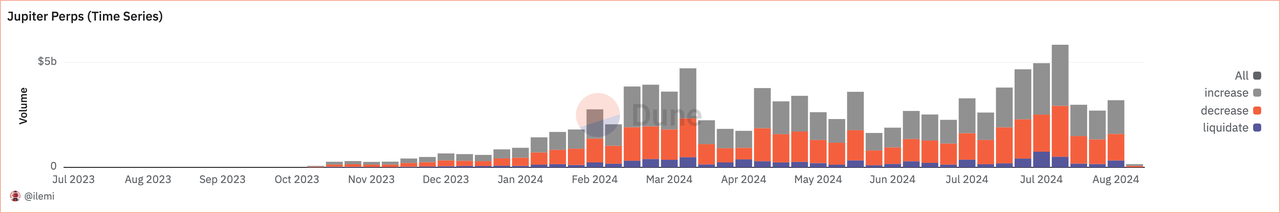
We can obtain Jupiter Perps trading volume directly from on-chain data.
Below is the DEX trading volume on Solana:
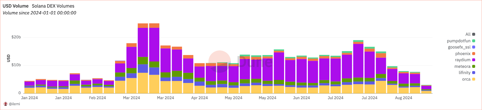
We see that Jupiter Perps' trading volume follows a similar trend to overall Solana DEX volume, yet exhibits stronger independence. Even as general volumes dropped sharply starting in July, Jupiter Perps maintained relatively solid levels.
Thus, while short-term volume forecasts can be accurately derived from on-chain analytics, long-term predictions must consider both Solana’s overall volume trends (beta) and Jupiter Perps’ own product-driven growth potential (alpha).
2. JLP’s TVL Scale
Having examined fee structure, let’s now turn to TVL—the total capital supplying leverage and sharing yield returns. The chart below shows steady growth in JLP’s TVL. Jupiter’s team adopts a prudent scaling strategy, setting an AUM Limit to control JLP size and mitigate excessive TVL swings that could destabilize LP returns—an approach reflecting strong operational responsibility.
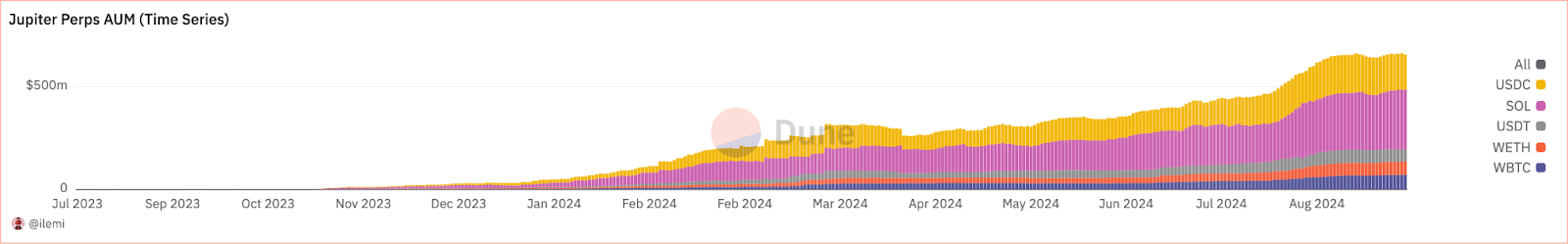
Overall, as JLP’s TVL cap continues to rise, its APY mean will inevitably trend downward. However, given the current bear market and a ~50% drop in market volume since July, a recovery in trading activity—combined with Jupiter Perps’ competitive edge—could drive JLP’s APY to rebound, potentially even surpassing 50%-60% again in the near term.
If you wish to estimate short-term APY—say, before official figures are released—you can visit RateX’s website. After mainnet launch, clicking on JLP contracts under Market Overview will give you access to leading-edge APY estimates for JLP.
3. How to Profit from Predicting JLP’s APY?
If you’ve grasped the methodology above and find APY forecasting both engaging and manageable, read on to learn how to monetize this insight using RateX’s JLP yield trading features.
1. Leveraged speculation on future APY.
RateX is a leveraged interest rate trading protocol that enables yield speculation via synthetic YT-JLP tokens. Essentially, it creates a liquid market for JLP yield trading. Liquidity Providers deposit JLP into the pool, which then issues rebasing ST-JLP tokens representing principal + accrued yield.
ST-JLP grows in quantity based on the official APY, ensuring its value tracks JLP’s yield-adjusted growth. For each JLP deposited, LPs can mint one YT-JLP token representing the pure yield stream.
Using YT-JLP and ST-JLP, RateX establishes an automated market maker (AMM) pool. Traders who want to leveraged-long YT deposit margin (in JLP), and the protocol mints ST-JLP for them to buy YT-JLP from the AMM.
Conversely, to short YT, traders deposit JLP margin, and the protocol mints YT-JLP for them to purchase ST-JLP in the AMM.
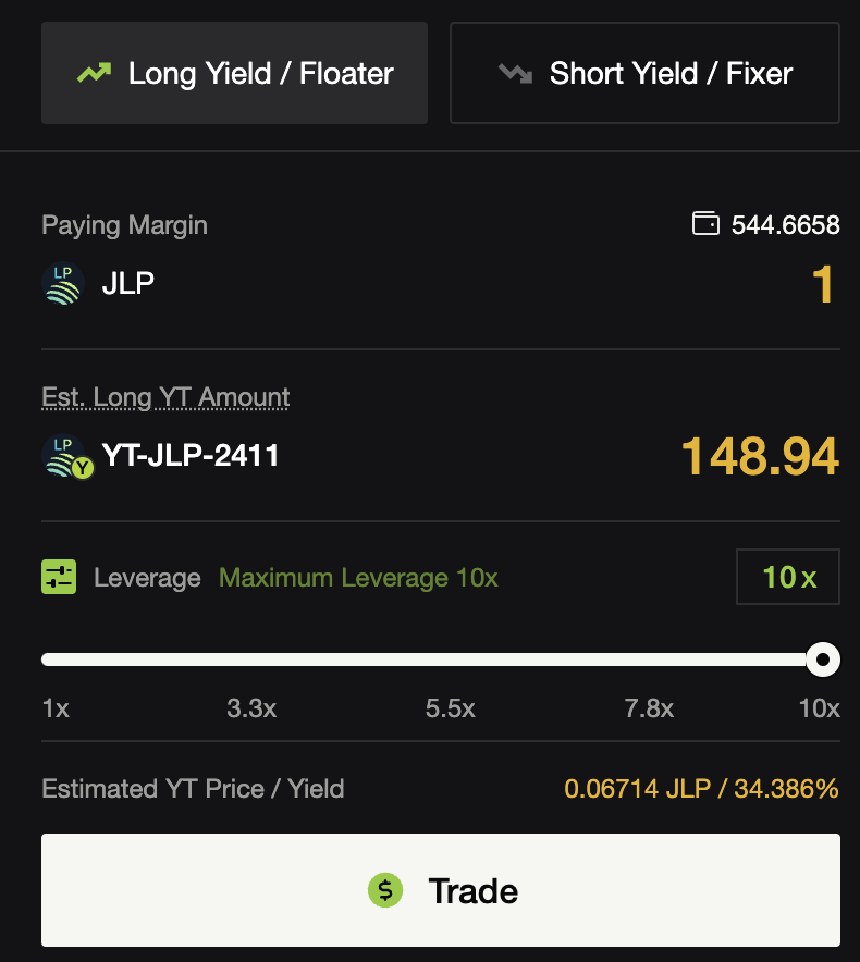
Currently, RateX supports up to 10x leverage on YT-JLP trades.
On RateX’s testnet, for the JLP-2411 contract (maturing end of November 2024), depositing 1 JLP of margin allows users to acquire 148.94 YT-JLP-2411 tokens.
YT price follows this formula:
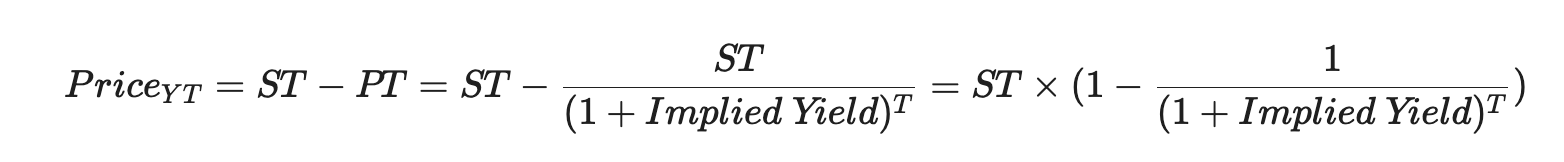
This nonlinear formula isn't intuitive. When implied yield is low, YT price changes roughly match the percentage change in implied yield (e.g., for a 6-month contract, implied yield rising from 3% to 4% results in ~33% price increase; from 30% to 40%, ~26% increase—due to discount factor sensitivity). Advanced users should compute exact values. A detailed explanation of YT tokens is available here.
2. Fixed-Income Investment
RateX constructs PT assets from YT and ST, where PT = 1 - YT. Since YT decays toward zero as yield accrues, PT converges in value toward one ST-JLP. Holding PT to maturity guarantees a fixed return—a conservative, passive yield strategy.
You can also pursue spread strategies with PT: if YT prices fall (implied yield drops), PT rises in value, allowing early redemption for higher effective annualized returns.
Alternatively, adopt a Kamino-style multiply strategy: collateralize PT, borrow funds, and reinvest into more PT for amplified returns. However, leverage introduces liquidation risk, so caution is advised.
3. Arbitrage Trading
Another strategy involves arbitrage based on predicting APY within a yield payment cycle. Since YT is a time-decaying asset, its value amortizes according to implied yield. At each payout period, YT is revalued. If the reduction in YT value doesn’t match the actual yield received, an arbitrage opportunity arises.
Suppose you buy YT at a 30% implied yield. In the next payout cycle, the realized APY is 50%, but your YT value depreciates only according to the 30% implied rate over time.
This means you earn more yield than the decline in YT value. If you immediately sell YT at market price, you capture arbitrage profit from correctly predicting the APY. However, such short-term arbitrage windows are narrow. Moreover, YT’s implied yield reflects market expectations of average APY over the remaining term, meaning failed arbitrage attempts may simply feed profits to longer-term traders. Hence, this strategy is not recommended unless you’re a professional trader.
If you found this article helpful, follow us on Twitter: @RateX_Dex to stay updated on more yield trading opportunities.
Join TechFlow official community to stay tuned
Telegram:https://t.me/TechFlowDaily
X (Twitter):https://x.com/TechFlowPost
X (Twitter) EN:https://x.com/BlockFlow_News