





Vitalik: Binius, efficient proofs for binary fields
TechFlow Selected TechFlow Selected
Vitalik: Binius, efficient proofs for binary fields
Binius is a proof system based on binary fields, designed to improve the efficiency of cryptographic proofs, particularly those related to SNARKs and STARKs.
 Navigating Web3 tides with focused insights
Author: Vitalik Buterin
Translation: Kate, Mars Finance
This article is primarily aimed at readers generally familiar with cryptography circa 2019, particularly SNARKs and STARKs. If you aren't, I recommend reading those articles first. Special thanks to Justin Drake, Jim Posen, Benjamin Diamond, and Radi Cojbasic for feedback and comments.
Over the past two years, STARKs have become a key and irreplaceable technology for efficiently creating easily verifiable cryptographic proofs about very complex statements (e.g., proving that an Ethereum block is valid). One key reason is field size: elliptic curve-based SNARKs require working over 256-bit integers for sufficient security, while STARKs allow smaller field sizes, which are more efficient—first the Goldilocks field (64-bit integers), then Mersenne31 and BabyBear (both 31-bit). Due to these efficiency gains, Plonky2 using Goldilocks is hundreds of times faster than its predecessors in proving various computations.
A natural question arises: can we take this trend to its logical conclusion by building even faster proof systems that operate directly on zeros and ones? This is exactly what Binius attempts to do, using many mathematical tricks that make it radically different from SNARKs and STARKs three years ago. This article introduces why small fields make proof generation more efficient, why binary fields have uniquely powerful properties, and the tricks Binius uses to make proofs over binary fields so effective.

Binius. By the end of this article, you should understand every part of this diagram.
Recap: Finite Fields
One key task of cryptographic proof systems is operating on large amounts of data while keeping numbers small. If you can compress a statement about a large program into a mathematical equation containing just a few numbers, but those numbers are as large as the original program, you've gained nothing.
To perform complex arithmetic while keeping numbers small, cryptographers usually use modular arithmetic. We pick a prime "modulus" p. The % operator means "take remainder": 15%7=1, 53%10=3, etc. (Note answers are always non-negative, so for example -1%10=9)

You may have already seen modular arithmetic in the context of adding/subtracting time (e.g., what time is 4 hours after 9?). But here, we don't just add and subtract modulo some number—we can also multiply, divide, and exponentiate.
We redefine:
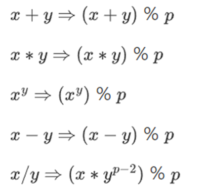
All the above rules are self-consistent. For example, if p=7, then:
5+3=1 (because 8%7=1)
1-3=5 (because -2%7=5)
2*5=3
3/5=2
The more general term for this structure is a finite field. A finite field is a mathematical structure that follows normal arithmetic laws but has a finite number of possible values, so each value can be represented with fixed size.
Modular arithmetic (or prime fields) is the most common type of finite field, but there's another type: extension fields. You might have encountered an extension field before: complex numbers. We "imagine" a new element and label it i, then do math with it: (3i+2)*(2i+4)=6i*i+12i+4i+8=16i+2. We can similarly take extensions of prime fields. As we start working with smaller fields, extensions of prime fields become increasingly important for maintaining security, and binary fields (used by Binius) rely entirely on extensions to be practically useful.
Recap: Arithmetization
SNARKs and STARKs prove computer programs via arithmetization: you convert a statement about a program you want to prove into a mathematical equation involving polynomials. Valid solutions to the equation correspond to valid executions of the program.
For a simple example, suppose I compute the 100th Fibonacci number and want to prove what it is. I create a polynomial F encoding the Fibonacci sequence: so F(0)=F(1)=1, F(2)=2, F(3)=3, F(4)=5, and so on for 100 steps. The condition I need to prove is F(x+2)=F(x)+F(x+1) across the range x={0,1,...98}. I can convince you by providing the quotient:
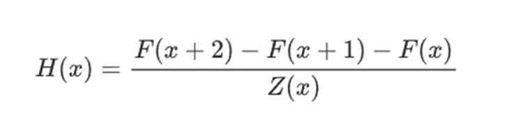
where Z(x) = (x-0) * (x-1) * ... * (x-98). If I can provide F and H satisfying this equation, then F must satisfy F(x+2)-F(x+1)-F(x) across that range. If I additionally verify F satisfies F(0)=F(1)=1, then F(100) must actually be the 100th Fibonacci number.
To prove something more complex, you replace the "simple" relation F(x+2) = F(x) + F(x+1) with a more complex equation that essentially says "F(x+1) is the output of initializing a virtual machine with state F(x) and running one computation step." You could also replace the number 100 with a larger number like 100,000,000 to accommodate more steps.
All SNARKs and STARKs are based on the idea of using simple equations over polynomials (sometimes vectors and matrices) to represent massive relationships between individual values. Not all algorithms check equivalences between adjacent computation steps like the above: for example, PLONK doesn't, nor does R1CS. But many of the most efficient checks do this because repeatedly performing the same check (or same few checks) makes it easier to minimize overhead.
Plonky2: From 256-bit SNARKs and STARKs to 64-bit... Only STARKs
Five years ago, a reasonable summary of different types of zero-knowledge proofs was: there are two types—elliptic curve-based SNARKs and hash-based STARKs. Technically, STARKs are a type of SNARK, but in practice "SNARK" usually refers to the elliptic curve variants while "STARK" refers to hash-based constructions. SNARKs are small, so you can verify them very quickly and easily put them on-chain. STARKs are large, but they don't require trusted setup and are quantum-resistant.
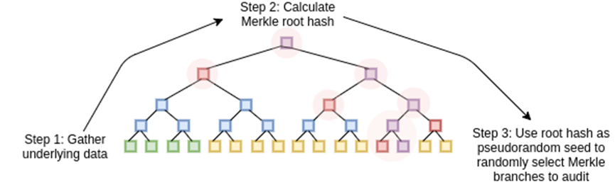
STARKs work by treating data as polynomials, computing evaluations of those polynomials, and using the Merkle root of the extended data as a "polynomial commitment"
A key historical point is that elliptic curve-based SNARKs were widely adopted first: STARKs didn't become efficient enough until around 2018 thanks to FRI, by which time Zcash had already been running for over a year. Elliptic curve-based SNARKs have a key limitation: if you use them, the arithmetic in these equations must be done modulo the number of points on the elliptic curve. This is a huge number, typically close to 2^256—for example, the bn128 curve uses 21888242871839275222246405745257275088548364400416034343698204186575808495617. But actual computations use small numbers: if you consider a "real" program in your favorite language, most things it uses are counters, loop indices, positions in the program, single bits representing True or False, and other things that are almost always only a few bits long.
Even if your "raw" data consists of "small" numbers, the proving process requires computing quotients, extensions, random linear combinations, and other data transformations, resulting in equal or greater quantities of objects whose average size is as large as your entire field size. This creates a key inefficiency: to prove computation over n small values, you must perform more computation over n much larger values. Initially, STARKs inherited SNARKs' habit of using 256-bit fields and thus suffered the same inefficiency.

Reed-Solomon extension of some polynomial evaluations. Despite original values being small, extra values all expand to full field size (in this case 2^31-1)
In 2022, Plonky2 was released. Plonky2's main innovation was doing arithmetic modulo a smaller prime: 2^64 - 2^32 + 1 = 18446744067414584321. Now every addition or multiplication can always be done in a few CPU instructions, and hashing all data together is 4x faster than before. But there's a problem: this approach only works for STARKs. If you try to use SNARKs, elliptic curves this small would be insecure.
To maintain security, Plonky2 also needed to introduce extension fields. A key technique for checking arithmetic equations is "random point sampling": if you want to check whether H(x)*Z(x) equals F(x+2)-F(x+1)-F(x), you randomly pick a coordinate r, open polynomial commitments to prove H(r), Z(r), F(r), F(r+1), and F(r+2), then verify whether H(r)*Z(r) equals F(r+2)-F(r+1)-F(r). If an attacker could guess the coordinate in advance, they could fool the proof system—that's why the proof system must be random. But this also means coordinates must be sampled from a sufficiently large set so attackers can't guess randomly. If the modulus is near 2^256, this is clearly true. But for modulus 2^64-2^32+1, we're not quite there, and definitely not if we go down to 2^31-1. Trying to forge a proof 2 billion times until someone gets lucky is absolutely within attackers' capabilities.
To prevent this, we sample r from an extension field—for example, define y where y^3=5, and use combinations of 1, y, y^2. This increases the total number of coordinates to around 2^93. Most of the polynomials computed by the prover don't enter this extension field; they just use integers modulo 2^31-1, so you still get all the efficiency benefits of using a small field. But the random point checks and FRI computations do go deep into this larger field to achieve required security.
From Small Primes to Binary
Computers do arithmetic by representing larger numbers as sequences of 0s and 1s and building "circuits" on top of these bits to compute operations like addition and multiplication. Computers are especially optimized for 16-bit, 32-bit, and 64-bit integers. For instance, 2^64-2^32+1 and 2^31-1 were chosen not just because they fit these bounds but because they align well with them: multiplication modulo 2^64-2^32+1 can be performed by doing regular 32-bit multiplications and bit-shifting/copying outputs in a few places; this article explains some of these tricks well.
However, an even better approach is computing directly in binary. What if addition could "just" be XOR without worrying about "carry" overflow from adding 1+1 on one bit to the next? What if multiplication could be similarly parallelized? These advantages come from being able to represent true/false values with a single bit.
Achieving these benefits of direct binary computation is exactly what Binius tries to do. The Binius team demonstrated efficiency gains in their zkSummit presentation:
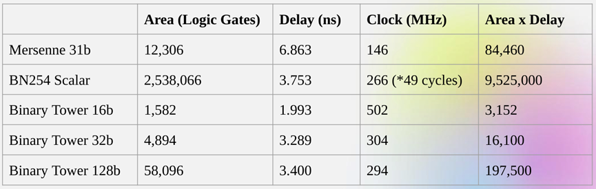
Despite "size" being roughly similar, 32-bit binary field operations require 5x fewer computational resources than 31-bit Mersenne field operations.
From Univariate Polynomials to Hypercubes
Suppose we accept this reasoning and want to do everything with bits (0s and 1s). How do we represent a billion bits with a polynomial?
Here we face two practical problems:
1. For a polynomial representing many values, those values need to be accessible during polynomial evaluation: in the Fibonacci example above, F(0), F(1)...F(100); in larger computations, exponents reach millions. Our field needs to contain numbers up to this size.
2. Any values we commit to in a Merkle tree (like all STARKs) need Reed-Solomon encoding: for example, extending n values to 8n, using redundancy to prevent malicious provers from cheating by forging one value during computation. This also requires a sufficiently large field: to extend a million values to 8 million, you need 8 million distinct points to evaluate the polynomial.
A key idea in Binius is solving these two problems separately and achieving this by representing the same data in two different ways. First, the polynomial itself. Elliptic curve-based SNARKs, 2019-era STARKs, Plonky2, and similar systems typically handle polynomials in one variable: F(x). Binius, inspired by the Spartan protocol, instead uses multivariate polynomials: F(x1,x2,...,xk). In practice, we represent the entire computation trace on a "hypercube" where each xi is either 0 or 1. For example, if we want to represent a Fibonacci sequence and still use a large enough field to represent them, we could imagine the first 16 numbers like this:
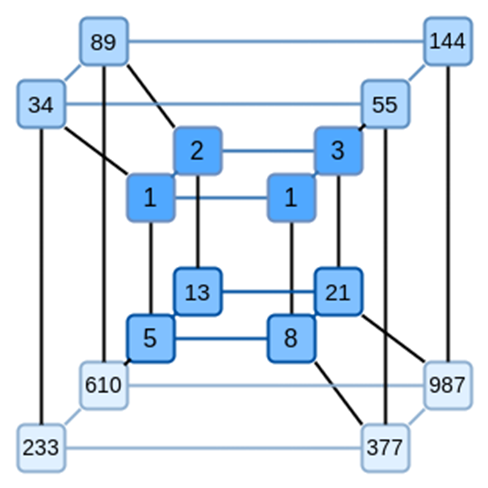
That is, F(0,0,0,0) should be 1, F(1,0,0,0) should also be 1, F(0,1,0,0) should be 2, and so on up to F(1,1,1,1)=987. Given such a hypercube of computations, there exists a multilinear (degree 1 in each variable) polynomial producing these values. So we can view this set of values as representing the polynomial; we don't need to compute coefficients.
Of course, this example is purely illustrative: in practice, the whole point of using hypercubes is to let us handle individual bits. A "Binius-native" way to compute Fibonacci numbers would use a high-dimensional cube storing one number per group of say 16 bits. This requires some cleverness to implement integer addition bit-by-bit, but isn't too difficult for Binius.
Now, let's look at erasure coding. STARKs work by: taking n values, Reed-Solomon extending them to more values (usually 8n, typically between 2n and 32n), then randomly selecting some Merkle branches from the extension and performing some check on them. A hypercube has length 2 in each dimension. So directly extending it isn't practical: there's not enough "space" to sample Merkle branches from 16 values. So what do we do? We pretend the hypercube is a square!
Simple Binius—An Example
See here for a Python implementation of the protocol.
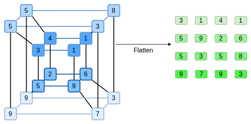
Let's look at an example, using regular integers as our field for convenience (in actual implementations, binary field elements would be used). First, we encode the hypercube we want to commit to as a square:
Now, we Reed-Solomon extend the square. That is, we treat each row as a degree-3 polynomial evaluated at x={0,1,2,3}, and evaluate the same polynomial at x={4,5,6,7}:
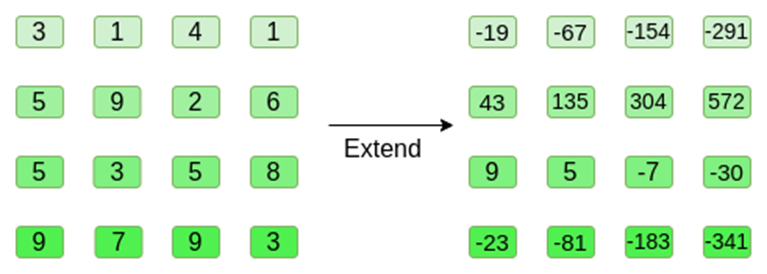
Notice how numbers blow up quickly! This is why in actual implementations we always use finite fields instead of regular integers: if we used integers modulo 11, for example, the first row's extension would just be [3,10,0,6].
If you want to try extending and personally verify the numbers here, you can use my simple Reed-Solomon extension code.
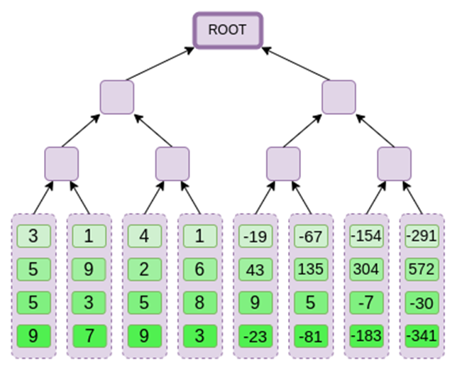
Next, we treat this extension as columns and create a Merkle tree of the columns. The Merkle root is our commitment.
Now, suppose the prover wants to prove the polynomial's evaluation at some point r={r0,r1,r2,r3}. There's a subtle difference in Binius making it weaker than other polynomial commitment schemes: the prover shouldn't know or be able to guess s before committing to the Merkle root (in other words, r should be a pseudorandom value depending on the Merkle root). This makes the scheme useless for "database lookups" (e.g., "Okay, you gave me the Merkle root, now prove P(0,0,1,0)!"). But the zero-knowledge proof protocols we actually use typically don't need "database lookups"; they only need to check polynomials at random evaluation points. So this limitation fits our purposes.
Suppose we choose r={1,2,3,4} (the polynomial evaluates to -137 at this point; you can confirm using this code). Now we enter the proof process. We split r into two parts: the first part {1,2} represents linear combinations of columns within rows, the second part {3,4} represents linear combinations of rows. We compute a "tensor product" for the column part:
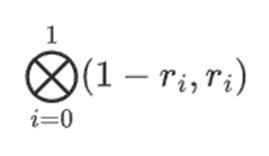
For the row part:
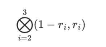
This means: the list of all possible products taking one value from each set. In the row case, we get:
[(1-r2)*(1-r3), (1-r3), (1-r2)*r3, r2*r3]
Using r={1,2,3,4} (so r2=3 and r3=4):
[(1-3)*(1-4), 3*(1-4),(1-3)*4,3*4] = [6, -9, -8, -12]
Now we compute a new "row" t by taking linear combinations of existing rows. That is, we take:
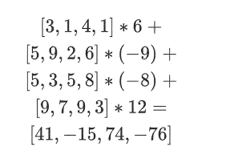
You can think of what's happening here as partial evaluation. If we multiplied the full tensor product by the full vector of all values, you'd get the evaluation P(1,2,3,4) = -137. Here, we multiply by only half the evaluation coordinates' partial tensor product, reducing the N-value grid to a row of √N values. If you give this row to someone else, they can complete the remaining calculation using the tensor product of the other half of evaluation coordinates.

The prover provides the following to the verifier: the new row t and Merkle proofs for some randomly sampled columns. In our illustrative example, we'll let the prover provide only the last column; in real life, the prover would need to provide dozens of columns for sufficient security.
Now we leverage linearity of Reed-Solomon codes. The key property we use is: taking a linear combination of Reed-Solomon extensions gives the same result as Reed-Solomon extending a linear combination. This "order independence" typically happens when both operations are linear.
The verifier does exactly this. They compute t and compute the same linear combination of columns the prover previously computed (but only for columns provided by the prover), then verify both processes give the same answer.
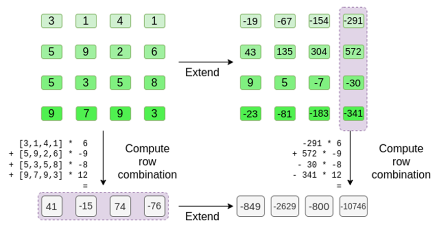
In this case, extending t and computing the same linear combination ([6,-9,-8,12]) both give the same answer: -10746. This proves the Merkle root was built "honestly" (or at least "close enough") and matches t: at least most columns are mutually compatible.
But the verifier also needs to check one more thing: verifying the polynomial's evaluation at {r0...r3}. So far, all the verifier's steps haven't actually depended on the value claimed by the prover. We check this as follows. We take the tensor product of the "column part" we labeled as the evaluation point:

In our example, where r={1,2,3,4} so the half selecting columns is {1,2}), this equals:

Now we take this linear combination of t:

This gives the same result as directly evaluating the polynomial.
The above is very close to a complete description of the "simple" Binius protocol. This already has some interesting advantages: for example, since data is split into rows and columns, you only need a field half the size. But it doesn't achieve all the benefits of computing in binary. For that, we need the full Binius protocol. But first, let's dive deeper into binary fields.
Binary Fields
The smallest possible field is arithmetic modulo 2, so small we can write out its addition and multiplication tables:

We can get larger binary fields through extension: starting from F2 (integers mod 2) and defining x where x^2=x+1, we get the following addition and multiplication tables:
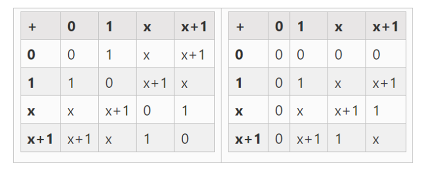
It turns out we can extend binary fields to arbitrarily large sizes by repeating this construction. Unlike complex numbers over reals, where you can add one new element but no more (quaternions do exist but are mathematically weird, e.g., ab ≠ ba), with finite fields you can keep adding new extensions indefinitely. Specifically, we define elements as follows:
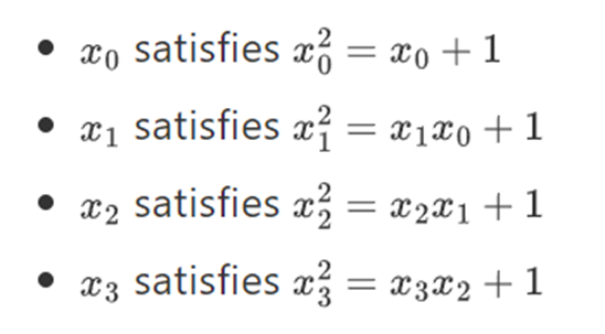
And so on... This is often called a tower structure because each successive extension can be seen as adding a new layer to the tower. This isn't the only way to construct binary fields of arbitrary size, but it has unique advantages that Binius exploits.
We can represent these numbers as lists of bits. For example, 1100101010001111. The first bit represents multiples of 1, the second multiples of x0, then subsequent bits represent multiples of the following x1 numbers: x1, x1*x0, x2, x2*x0, and so on. This encoding is nice because you can decompose it:
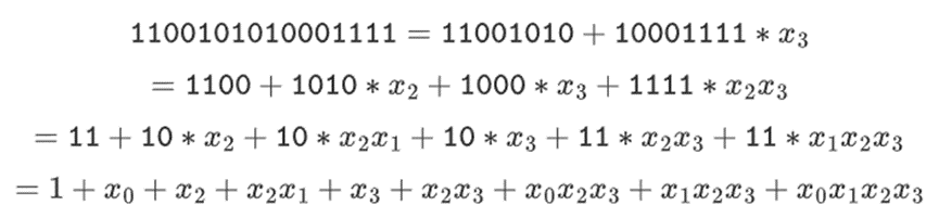
This is a relatively uncommon notation, but I like representing binary field elements as integers using bit representation with more significant bits on the right. That is, 1=1, x0=01=2, 1+x0=11=3, 1+x0+x2=11001000=19, etc. In this notation, it's 61779.
Addition in binary fields is just XOR (subtraction is too, by the way); note this means x+x=0 for any x. Multiplying two elements x*y has a very simple recursive algorithm: split each number in half:

Then split the multiplication:

The last part is the only slightly tricky bit, as you must apply simplification rules. There are more efficient ways to do multiplication, analogous to Karatsuba algorithm and Fast Fourier Transform, but I'll leave that as an exercise for interested readers to figure out.
Division in binary fields is done via multiplication combined with inversion. The "simple but slow" inversion method applies the generalized Fermat's little theorem. There's a more complex but more efficient inversion algorithm you can find here. You can play with binary field addition, multiplication, and division using the code here.
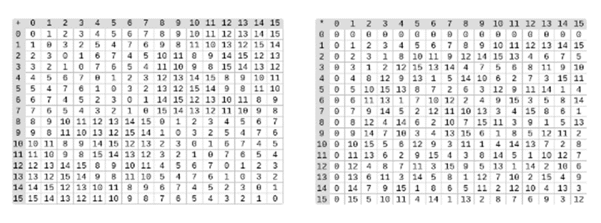
Left: Addition table for four-bit binary field elements (i.e., composed only of 1, x0, x1, x0x1). Right: Multiplication table for four-bit binary field elements.
The beauty of this type of binary field is it combines some of the best aspects of "regular" integers and modular arithmetic. Like regular integers, binary field elements are unbounded: you can extend them as much as you want. But like modular arithmetic, if you operate on values within a certain size limit, all your results stay within that same range. For example, taking powers of 42 continuously, you get:

After 255 steps, you return to 42^255=1. Like regular integers and modular arithmetic, they follow normal mathematical laws: a*b=b*a, a*(b+c)=a*b+a*c, and even gain some strange new laws.
Finally, binary fields handle bits conveniently: if you do math with numbers fitting in 2^k, all your outputs will also fit in 2^k bits. This avoids awkwardness. In Ethereum's EIP-4844, the various "chunks" of a blob must be numbers modulo 52435875175126190479447740508185965837690552500527637822603658699938581184513, so encoding binary data requires wasting space and extra application-layer checks to ensure each element stores a value less than 2^248. It also means binary field operations are super fast on computers—whether CPUs or theoretically optimal FPGA and ASIC designs.
All this means we can do Reed-Solomon encoding like above in a way that completely avoids integer "explosion" as we saw in our example, and in a very "native" way that computers excel at. The "splitting" property of binary fields—how we did 1100101010001111=11001010+10001111*x3 and can split further as needed—is also crucial for achieving great flexibility.
Full Binius
See here for a Python implementation of the protocol.
Now we can move to "full Binius," which adapts "simple Binius" to (i) work over binary fields and (ii) let us commit to individual bits. This protocol is hard to understand because it keeps switching between different ways of viewing bit matrices; certainly, it took me longer to understand it than I usually spend on cryptographic protocols. But once you understand binary fields, the good news is there's no "harder math" that Binius relies on. No elliptic curve pairings with ever-deeper algebraic geometry rabbit holes to explore; here, you only need binary fields.
Let's look at the full diagram again:

By now, you should be familiar with most components. The ideas of flattening the hypercube into a grid, computing row and column combinations as tensor products of evaluation points, and testing equivalence between "Reed-Solomon extend then compute row combination" and "compute row combination then Reed-Solomon extend" were all implemented in simple Binius.
What's new in "full Binius"? Essentially three things:
• Individual values in the hypercube and square must be bits (0 or 1).
Join TechFlow official community to stay tuned
Telegram:https://t.me/TechFlowDaily
X (Twitter):https://x.com/TechFlowPost
X (Twitter) EN:https://x.com/BlockFlow_News
 @VitalikButerin