Dissecting the Uniswap V3 Data Cleaning Process
TechFlow Selected TechFlow Selected
Dissecting the Uniswap V3 Data Cleaning Process
We calculated user net worth and return rates on Uniswap from the perspective of user addresses.
Author: Zelos
Introduction
In the previous article, we analyzed users' net value and returns on Uniswap from the perspective of user addresses. This time, our goal remains the same—but now we will also include cash holdings in these addresses to calculate an overall net value and return rate.
We focus on two liquidity pools:
-
USDC-WETH (fee: 0.05%) on Polygon, pool address: 0x45dda9cb7c25131df268515131f647d726f50608[1], which is the same pool used in the last analysis
-
USDC-ETH (fee: 0.05%) on Ethereum, pool address: 0x88e6A0c2dDD26FEEb64F039a2c41296FcB3f5640[2]. Since this pool involves a native token, it introduces some complexity in data processing
The final dataset is hourly. Note: each row represents the value at the end of that hour.
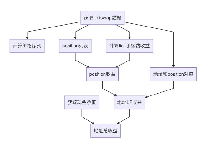
Overall Workflow
-
Obtain Uniswap data
-
Obtain user cash holding data
-
Calculate price series (i.e., ETH price)
-
Determine fee earnings per minute for each tick
-
Retrieve list of all positions during the analysis period
-
Map addresses to their corresponding positions
-
Calculate return rate for each position
-
Based on the mapping between positions and addresses, compute LP return rates for each user address
-
Combine user cash and LP holdings to compute overall returns
1. Obtaining Uniswap Data
Previously, we developed a tool called demeter-fetch to provide data sources for Demeter. This tool can fetch logs from various Uniswap pools via multiple channels and parse them into different formats. Supported data sources include:
-
Ethereum RPC: Standard RPC interface from Ethereum clients. Data retrieval is relatively slow, requiring multi-threading for efficiency.
-
Google BigQuery: Download data from public datasets. Although updated daily, it's convenient and cost-effective.
-
Trueblocks Chifra: The Chifra service scrapes on-chain transactions and reorganizes them, allowing easy export of transaction and balance information. However, this requires setting up your own node and service.
Output formats supported:
-
Minute-level: Resample Uniswap swap events into one-minute intervals, suitable for backtesting
-
Tick-level: Record every transaction in the pool, including swaps and liquidity operations
For this analysis, we primarily use tick-level data to capture detailed position information such as capital amount, per-minute returns, lifespan, and holders.
This data comes from the pool’s event logs—such as mint, burn, collect, and swap. However, pool logs do not contain token IDs, making it impossible to directly link operations to specific positions.
In reality, Uniswap LP positions are managed through NFTs, and these NFTs are controlled by a proxy contract. Token IDs only appear in the proxy contract’s event logs. Therefore, to obtain complete LP position details, we must combine logs from both the pool and the proxy contract.
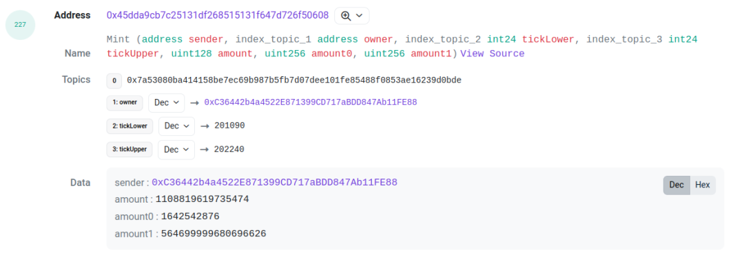
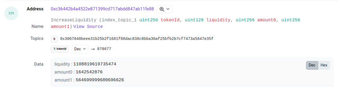
Take this transaction[3] as an example: We focus on log indices 227 and 229. Log 227 is the Mint event from the pool contract, while log 229 is the IncreaseLiquidity event from the proxy contract. Both share identical values for amount (liquidity), amount0, and amount1. This allows us to associate the two events. By linking them, we can determine the LP’s tick range, liquidity, token ID, and respective token amounts.
Advanced users, especially funds, may bypass the proxy and interact directly with the pool contract. In such cases, the position won’t have a token ID. For these, we create a synthetic ID using the format address-LowerTick-UpperTick.
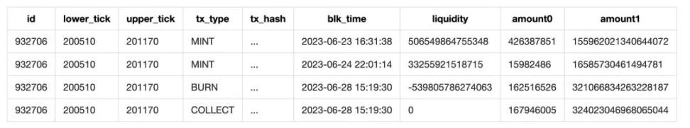
Similarly, for Burn and Collect events, we match pool events to positions using the same method. However, there’s a challenge: sometimes the amounts differ slightly between events. For instance:
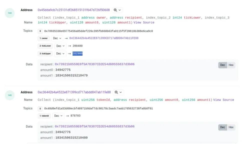
Here, amount0 and amount1 show minor discrepancies. While rare, such mismatches do occur. To handle this, we allow a small tolerance when matching Burn and Collect events.
Another issue is identifying who initiated the transaction. For withdrawals, we use the recipient in the Collect event as the position holder. For mints, we extract the sender from the pool’s Mint event (see image with mint event).
If the user interacts directly with the pool, the sender is the LP provider. But if they go through the proxy, the sender will be the proxy contract address—because funds are transferred from the proxy to the pool. Fortunately, the proxy generates an NFT token, which is always transferred to the actual LP provider. Thus, by monitoring transfers from the proxy (NFT) contract, we can identify the true LP provider behind each mint.
Additionally, if an NFT is transferred later, the position holder changes. We’ve observed such cases, but they’re infrequent. For simplicity, we ignore post-mint NFT transfers.
2. Obtaining Address Cash Holdings
The goal here is to determine how many tokens an address holds at each moment during the analysis period. To achieve this, we need two types of data:
-
Balance of the address at the start time
-
Transfer records of the address during the analysis period
By applying transfers to the initial balance, we can infer balances at any given time.
Initial balances can be queried via RPC. With an archive node, you can specify block height to retrieve historical balances. This works for both native tokens and ERC20s.
ERC20 transfer records are easy to obtain through any channel (BigQuery, RPC, Chifra).
However, ETH transfers require fetching transactions and traces. While transactions are manageable, processing traces is computationally intensive. Fortunately, Chifra offers a feature to export ETH balance changes—recording only when the balance changes, though without counterparty info. Despite this limitation, it meets our needs at minimal cost.
3. Price Derivation
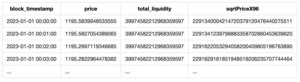
Uniswap is a DEX; whenever a token swap occurs, a Swap event is emitted. From the sqrtPriceX96 field, we can derive the token price. The liquidity field gives current total liquidity in the pool.
Since both pools contain a stablecoin, deriving USD prices is straightforward. However, this price isn’t perfectly accurate. First, it depends on swap frequency—without recent swaps, the price lags. Second, if the stablecoin de-pegs, the derived price diverges from its true USD value. Nevertheless, under normal conditions, this approximation is sufficient for market analysis.
Finally, resampling yields a per-minute price series.
Additionally, since the event’s liquidity field contains total pool liquidity, we include it in our output. The result is a table like this:
4. Fee Revenue Calculation
Fees are the primary income source for LPs. Every time a user performs a swap on the pool, positions whose tick ranges include the current tick earn fees. Earnings depend on the proportion of liquidity provided, the pool’s fee tier, and the tick range width.
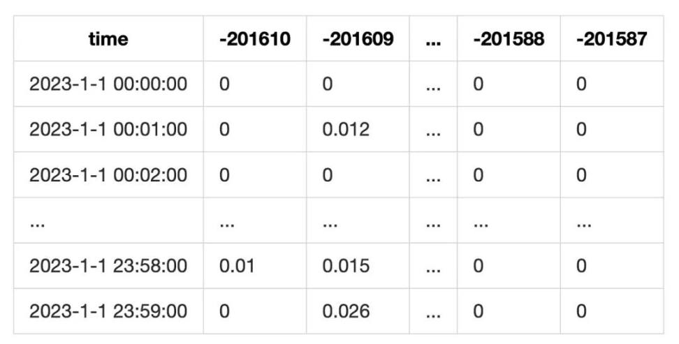
To track fee income, we record, for each minute, which tick had swaps and how much volume was traded. Then we compute fee revenue for that minute:

Resulting in a table like this:
This method doesn't account for scenarios where the current tick runs out of liquidity during a swap. However, since we're analyzing LPs using tick ranges, this error is partially mitigated.
5. Retrieving Position List
To compile a list of positions, we first define a unique identifier for each:
-
For LPs using the proxy, each position has an NFT with a token ID, which serves as the position ID.
-
For direct pool interactors, we generate a synthetic ID in the format
address_LowerTick_UpperTick. This ensures all positions have a unique identifier.
Using these IDs, we aggregate all actions related to a position into a full lifecycle timeline, such as:
Note: Our analysis covers only 2023, not from the pool’s inception. Therefore, for some positions, we lack pre-2023 activity data. We must estimate their initial liquidity at the start of 2023. We adopt a practical approach:
-
Sum up all minted and burned liquidity to get a net value L
-
If L > 0 (more minted than burned), assume existing liquidity before 2023. Add a synthetic mint event at the start of 2023 (Jan 1, 00:00:00).
-
If L < 0, assume residual liquidity remains at year-end.
This avoids downloading pre-2023 data, saving costs. However, it introduces the issue of "sunken liquidity"—LPs who made no activity in 2023 won’t be detected. But this isn’t severe. Given the one-year span, most active users adjust their positions due to price movements or reallocating funds. Truly inactive LPs are excluded from our scope.
A more problematic case: a position minted liquidity before 2023, performed some mints/burns during the year, but didn’t fully withdraw by year-end. We’d only observe part of its liquidity, leading to inaccurate fee estimates and distorted returns. We’ll discuss this further later.
Ultimately, we identified 73,278 positions on Polygon and 21,210 on Ethereum, with fewer than 10 anomalous returns per chain—validating our assumptions.
6. Mapping Addresses to Positions
Since our ultimate goal is measuring address-level returns, we need to map addresses to positions. This linkage enables understanding individual investment behaviors.
As discussed in Step 1, we already traced fund operators (via mint senders and collect recipients). Thus, identifying the sender of a mint or the recipient of a collect gives us the address-position mapping.
7. Calculating Position Net Value and Return Rate
Here, we compute net value for each position, then derive return rates from those values.
Net Value
A position’s net value consists of two parts: (1) liquidity, representing the principal invested. Once deposited, the liquidity amount stays constant, but its USD value fluctuates with price. (2) Fee income, stored separately in fee0 and fee1 fields, grows over time independently of liquidity.
At any minute, combining liquidity with the current price gives the principal’s net value. Fee income relies on the fee table computed earlier.
First, divide the position’s liquidity by total pool liquidity to get its share. Then sum fees across all ticks within the position’s tick range to get that minute’s fee earnings.
Mathematically:

Summing fee0 and fee1 gives total fee value. Adding this to the liquidity value yields total net value.
We segment a position’s lifecycle based on mint/burn/collect transactions:
-
On mint: increase liquidity
-
On burn: decrease liquidity. Convert remaining liquidity value into fee fields (matching pool contract logic)
-
On collect: trigger calculation from last collect to current time, computing net value and fee income per minute, resulting in a time-series list
Finally, merge all collect-triggered lists, resample, and perform further aggregation to produce final results.
We implemented two optimizations for higher accuracy:
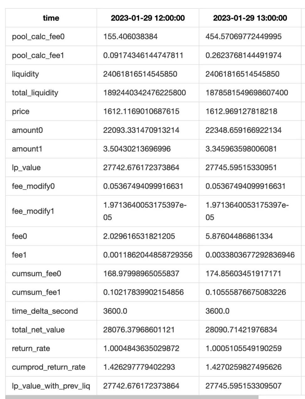
First, for hours with transactions (mint/burn/collect), we perform minute-level tracking; for inactive hours, we use hourly resolution, then resample everything to hourly.
Second, Collect events reveal the total of liquidity + fees. Comparing actual collected amounts against our theoretical calculations gives a discrepancy (which also includes tiny LP principal differences, negligible in practice). We distribute this difference across rows to improve fee estimation accuracy (see fee_modify0 and fee_modify1 in the table above).
Notes:
-
When backfilling, weight fee allocation by current hour’s liquidity share—otherwise, fees may appear inflated.
-
Due to partial data (only 2023), we face “sunken liquidity” issues (as mentioned in Section 5). This causes actual fees to exceed theoretical ones, inflating returns abnormally.
Since each row reflects the end-of-hour snapshot, closed positions show zero net value. This erases their final value. To preserve it, we append a record at 2038-01-01 00:00:00 containing the closing net value, useful for downstream analyses.
Return Rate
Typically, return rate = ending value / starting value. But this doesn’t work here because:
-
We need minute-level granularity,
-
Positions may have mid-period deposits/withdrawals. Simple division fails to reflect true performance.
For issue 1, we compute per-minute returns by dividing consecutive values, then compound them multiplicatively for total return:

But this has a serious flaw: a single incorrect minute skews the entire cumulative return. It makes error detection both critical and visible.
For issue 2, direct division still produces absurd returns when deposits/withdrawals occur. So we refine the per-minute algorithm.
Our first attempt splits net value changes into components: (1) price-driven principal change, (2) fee accrual, (3) fund inflows/outflows. Clearly, (3) should be excluded. Hence:
-
Let current minute be n, previous be n−1
-
Assume all transfers happen at n:00.000. Afterward, LP value remains constant until n:59.999
-
Fee accrual happens at minute end: n:59.999
-
End-of-(n−1) values become start-of-n values
Under these assumptions, per-minute return = (end liquidity × end price × end fees) / (end liquidity × start price × start fees). Formula below, where f converts liquidity to value:

This seems ideal—it isolates price and fee impacts, excluding liquidity changes. But in practice, extreme returns appear occasionally. Investigation reveals the problem lies in withdrawal timing. Recall: each row represents end-of-minute/hour values. But column semantics differ:
-
Net value: instantaneous (end-of-interval)
-
Fees: cumulative (total earned during interval)
So, during a burn hour:
-
After burning and withdrawing tokens, net value drops to 0
-
But fees remain positive—they accumulate throughout the hour
This reduces the formula to:
This isn’t limited to final burns—partial burns also distort fee-to-value ratios.
For simplicity, when LP value changes, we set return rate to 1. This introduces error, but for normally active positions, trading hours are few relative to lifespan—so impact is minimal.
8. Computing Aggregate LP Return per Address
With per-position returns and address mappings, we now compute each address’s LP return history.
Algorithm is simple: concatenate positions held by the address over time. Periods with no positions have net value = 0 and return = 1 (no change).
If multiple positions overlap, sum their net values. When merging returns, apply value-weighted averaging.
9. Combining Cash and LP Total Returns
Finally, combine cash holdings and LP investments for each address to get total net value and return.
Net value combination is simpler than merging positions. Just align LP net value timestamps, pull corresponding cash balances, apply ETH price, and sum.
For returns, we again use per-minute compounding. Initially, we tried the flawed method from Section 7—requiring separation of fixed (cash balances, LP liquidity) and variable (price moves, fee accrual, fund flows) components. This is far more complex than position-only analysis. For LPs, inflows/outflows are captured via mint/collect. But tracing cash flows is messy—we must distinguish whether funds went to LP or external addresses. If to LP, principal unchanged; if external, adjust principal. This requires tracking ERC20 and ETH transfer destinations—a huge task. Mint/collect might involve pool or proxy addresses. Worse, ETH transfers (native tokens) often require trace data, which exceeds our processing capacity.
The final straw came when we realized: net value (instantaneous) and fees (cumulative) cannot be meaningfully added per row—this distinction wasn’t clear until late.
Thus, we abandoned that method. Instead, we use (next minute net value) / (current minute net value). Simpler—but still breaks when fund flows occur. As shown earlier, separating flow directions is too hard. So we sacrifice precision: set return = 1 whenever fund transfers occur.
Now, how to detect fund inflows/outflows? Initial idea: use prior hour’s token balances and current price to predict what net value would be if unchanged. Compare prediction vs actual. Non-zero difference implies fund movement. Formula:

But this ignores Uniswap LP complexity: token amounts and net value change with price, and fees aren’t considered. Resulting in ~0.1% prediction error.
To improve accuracy, break down components: model LP value changes separately and include fees:

This reduces prediction error to within 0.001%.
Also, we cap decimal precision to avoid dividing extremely small numbers (typically <1e-10), which are artifacts of computation and resampling. Unchecked, such divisions amplify errors and distort returns.
Other Issues
Native Token
This analysis includes Ethereum’s USDC-ETH pool, where ETH is a native token requiring special handling.
ETH cannot be used directly in DeFi; it must be wrapped into WETH. Thus, this pool is effectively USDC-WETH. Direct pool interactors simply deposit/withdraw WETH—same as regular pools.
For proxy users, ETH is sent as transaction value to the proxy, which converts it to WETH before depositing. On collect, USDC goes directly to user; ETH must first exit pool to proxy, be unwrapped, then sent as native ETH. See example transaction[4].
Thus, USDC-ETH differs from standard pools only in fund flow mechanics—impacting only address-position mapping. To resolve, we extracted all NFT transfer logs since pool creation and mapped token IDs to position owners.
Missing Positions
Some positions don’t appear in final results due to special characteristics.
Many are MEV transactions—pure arbitrage, not typical investors, so excluded. Statistically challenging too, requiring trace-level data. We filter them simply: positions lasting less than one minute. Since our finest resolution is one minute, sub-minute positions are undetectable.
Another possibility: positions with no Collect events. As seen in Step 7, we compute returns triggered by collects. Without collects, no valuation occurs. Normally, users collect fees or principal periodically. But some may intentionally leave assets in fee0/fee1. These are edge cases, excluded from our analysis.
Join TechFlow official community to stay tuned
Telegram:https://t.me/TechFlowDaily
X (Twitter):https://x.com/TechFlowPost
X (Twitter) EN:https://x.com/BlockFlow_News