
BiB Exchange: The Liquidity Finance Miracle, Unveiling Hedging Logic and Mitigating Impermanent Loss Risk
TechFlow Selected TechFlow Selected
BiB Exchange: The Liquidity Finance Miracle, Unveiling Hedging Logic and Mitigating Impermanent Loss Risk
This article will delve into the core of liquidity, exploring how instruments such as options and perpetual contracts can serve as powerful tools in mitigating impermanent risk.
Author: BiB Exchange
Introduction
In the world of crypto, platforms such as Uniswap and Curve are undoubtedly shining stars in decentralized finance. However, when investors face impermanent loss, intelligently hedging this risk has become a crucial task. In this exploration of hedging logic, BiB Exchange dives into the core of liquidity to examine how instruments like options and perpetual contracts can serve as powerful tools to mitigate impermanent loss.
Liquidity Providers (LPs) represent one of the most common business models in the DeFi sector today. LPs supply capital to liquidity pools, enabling services such as earning trading fees, participating in yield farming, securing crypto loans, or transferring ownership of staked liquidity. At its core, this model operates under Automated Market Maker (AMM) algorithms. By depositing two or more tokens into a pool, LPs provide market liquidity and earn transaction fees. However, this approach often exposes them to the risk of impermanent loss.
This article by BiB Exchange is structured into three main sections: First, we introduce common AMM mechanisms and their characteristics; second, using Uniswap V2 as an example, we analyze impermanent loss and its mathematical properties; third, we explore several popular hedging strategies—dynamic hedging, perpetual power contracts, and options—and compare their advantages and disadvantages.
1. Understanding AMMs
Users who contribute funds to liquidity pools become Liquidity Providers (LPs). The underlying mechanism relies on Automated Market Makers (AMMs), more specifically known as Constant Function Market Makers (CFMMs). This system operates on decentralized platforms without requiring traditional intermediaries, supports multi-asset trading pairs, and exhibits several distinct features:
-
No Order Book: Unlike centralized exchanges, AMMs do not rely on bid-ask order books. Instead, trades execute directly through smart contracts rather than via order matching.
-
Trading Fees: Each trade incurs a fee paid to liquidity providers, calculated based on their share of the pool. This incentivizes users to supply more liquidity, enhancing market activity.
-
Continuous Price Adjustment: Asset prices adjust continuously according to supply and demand due to algorithmic pricing, enabling instant execution at available rates without waiting for order matching.
Currently, leading DEX platforms employ various AMM algorithms:
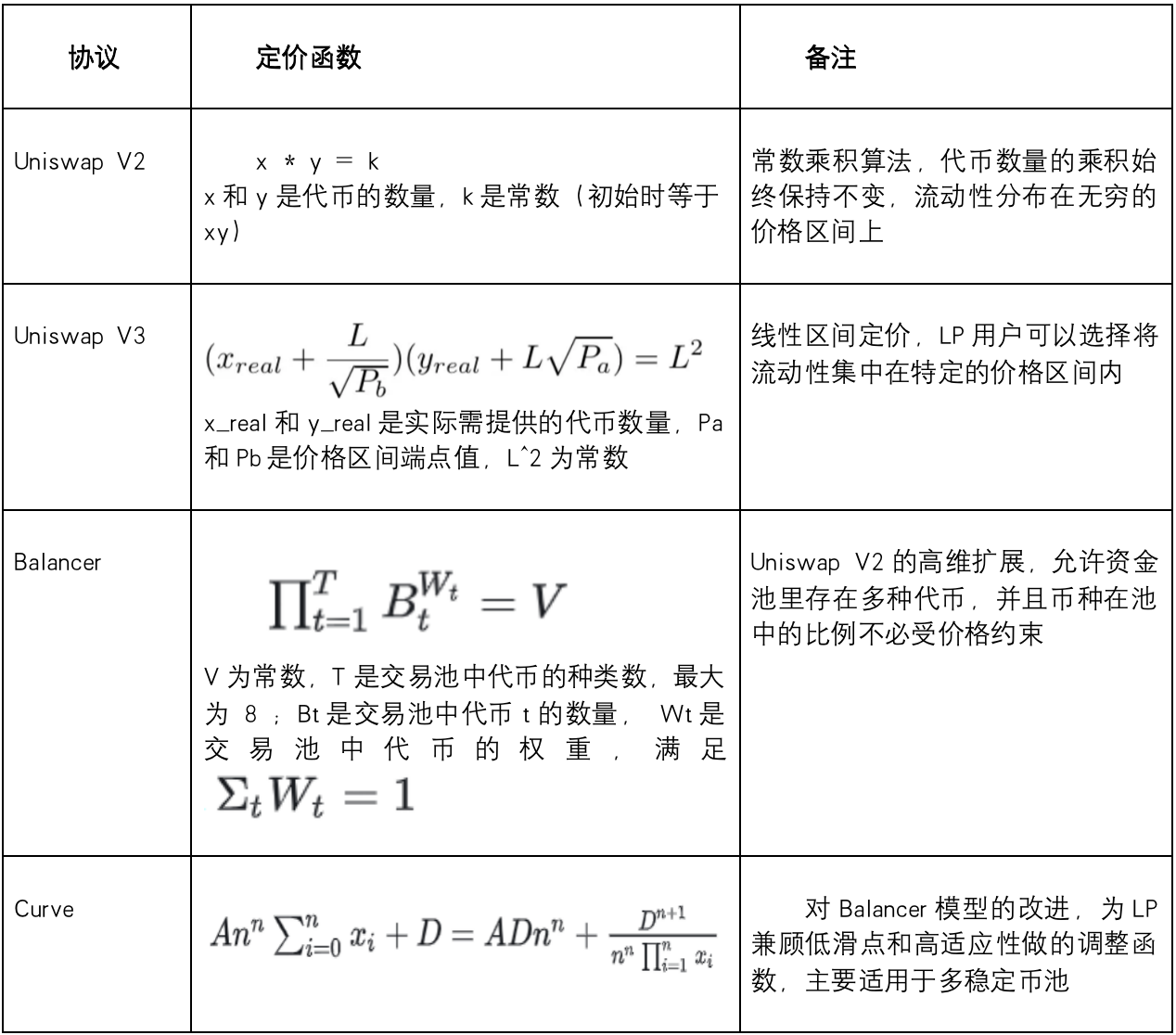
In these protocols, traders pay a percentage fee per transaction, part of which is distributed as rewards to LPs. However, due to impermanent loss, LPs must carefully balance earned fees against potential losses.
Meanwhile, during the period that LPs have assets deposited, any price fluctuation creates a discrepancy between the market price and the pool’s internal price, opening arbitrage opportunities. Arbitrageurs will continuously trade until the asset ratio aligns with the external market price. During this process, LPs earn fees from these trades, while arbitrageurs profit from price differences—this very mechanism results in potential losses for LPs, known as impermanent loss.
2. Functional Characteristics
Taking Uniswap V2's AMM mechanism as an example, BiB Exchange illustrates how impermanent loss occurs. It uses the formula X*Y=K to determine the relative value of two assets within a pool, where X and Y represent the quantities of each asset and K is a constant.
Assume a liquidity pool contains ETH and DAI. A user deposits 1 ETH and 100 DAI into the pool. Under the AMM model, deposited assets must be of equal value at the time of deposit, meaning 1 ETH = 100 DAI. Thus, the total value of the user’s deposit is $200. If the entire pool holds 10 ETH and 1,000 DAI, the total liquidity is $2,000, giving the user a 10% share. The constant K = 10 * 1,000 = 10,000.
Now suppose the spot price of ETH rises to 400 DAI, while the pool still reflects a price of 100 DAI. Arbitrageurs notice this mispricing and add DAI to the pool while removing ETH until the ratio approaches the market price. According to the constant product rule (K remains unchanged), the new state becomes approximately 5 ETH and 2,000 DAI (ignoring fees).
If the user now withdraws funds based on their 10% share, they receive 0.5 ETH and 200 DAI, totaling $400. While this appears profitable, had the user simply held onto 1 ETH and 100 DAI instead of providing liquidity, their holdings would now be worth $500. Therefore, the user incurs a $100 loss compared to holding—a phenomenon known as impermanent loss.
Note: This example ignores fees earned by being an LP.
Let us perform a simple derivation:
Define P as the price of ETH in terms of DAI: P = Y/X
From X*Y = K and P = Y/X, solving gives:
X = (K/P)^0.5; Y = (K*P)^0.5
For two points in time T0 and T1, with prices P0 and P1 respectively, let P1 = λP0, where λ is the price change multiplier.
At T1, the value of the LP position is: 2*Y1 = 2*(K*λP0)^0.5
If not providing liquidity, the original assets’ value would be: X0*P1 + Y0 = (1+λ)*(K*P0)^0.5
Impermanent Loss IL(λ) = [2*(K*λP0)^0.5 - (1+λ)*(K*P0)^0.5] / [(1+λ)*(K*P0)^0.5] = 2√λ/(1+λ) - 1
= -(√λ - 1)² / (1 + λ) ≤ 0 always holds true.
Thus, whenever the price changes, LPs inevitably suffer impermanent loss.
The following graph shows the function of impermanent loss across different price movements:
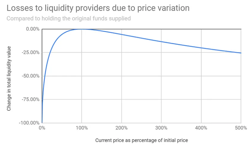
As shown, greater price volatility leads to larger impermanent losses compared to simply holding. However, if the collected fees exceed the impermanent loss, the LP can still remain profitable.
Other common AMM mechanisms exhibit similar functional behaviors—price fluctuations lead to impermanent loss. So how can it be avoided? Below, we explore possible solutions.
3. Hedging Impermanent Loss
Suppose a liquidity pool consists of ETH and DAI, and a user deposits 1 ETH and 100 DAI. At deposit time, both assets are valued equally: P = 100 / 1 = 100.
Using a 50% volatile asset / 50% stablecoin portfolio as a benchmark (though other benchmarks exist, such as holding only volatile assets), we’ll explore methods to hedge impermanent loss.
The value of a 50:50 portfolio is V_HODL_50(λ) = (1+λ)*(K*P0)^0.5—a linear function of price movement λ.
In contrast, the LP value function V_LP(λ) = 2*(K*λ*P0)^0.5 is a square root function—nonlinear. This nonlinearity exists across all reasonable AMM designs (with varying functional forms).
We introduce two key concepts:
-
Delta: The first derivative of the portfolio value with respect to price, representing sensitivity to price changes.
-
Gamma: The second derivative, measuring how delta itself changes with price.
Notably, the gamma of the HODL portfolio is always zero, whereas the LP portfolio has negative gamma.
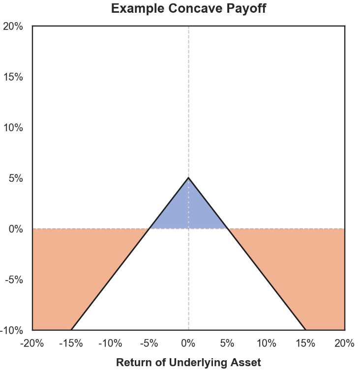
Negative Gamma Payoff: Profits decrease when prices rise, losses amplify when prices fall
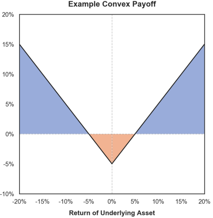
Positive Gamma Payoff
How do we address negative gamma exposure? BiB Exchange identifies several strategies:
1) Maximize fee income: When fees exceed impermanent loss, LPs profit. This involves selecting high-volume pools and optimal fee tiers, akin to active trading rather than passive investing. Metrics like implied volatility (IV) or Sharpe ratio may guide decisions.
2) Choose low-volatility pairs: Stablecoin pairs typically avoid impermanent loss but carry small depeg risks that could result in catastrophic losses.
3) Dynamically rebalance positions as prices shift.
4) Hedge using financial instruments with positive gamma, such as options or power perpetuals.
3.1 Perpetual Contracts
Maximizing fee income essentially means choosing the right pool and fee tier, and anticipating market movements—closer to trading than passive investment. Beyond APY, metrics like Implied Volatility (IV)—derived from option prices—or the Sharpe Ratio—measuring excess return per unit of risk—can inform better decisions.
Low-volatility pairs: Stable pairs usually avoid impermanent loss, though rare depeg events pose severe risks.
Dynamic hedging: Consider native DeFi strategies involving borrowing. Compared to perpetual-based hedging, this requires more upfront capital but is safer and easier to implement.
Alice starts with 5000 USDC and provides liquidity in a USDC/ETH pool. Initial ETH price: 1000 USDC.
She deposits 4000 USDC into Aave, borrows 1 ETH, and allocates assets in a 50:50 ratio into a full-range Uniswap position.
Initial capital: 5000 USDC, split into hedge (worth 3000 USDC) and pool (worth 2000 USDC):
V_collateral = 4000
V_debt = 1000 → V_hedge = 4000 – 1000 = 3000
V_capital = V_pool + V_hedge = 5000
When ETH doubles to 2000 USDC, the pool value becomes 2000·√2 ≈ 2828 USDC, but the hedge value drops to 2000 USDC:
V_collateral = 4000, V_debt = 2000 → V_hedge = 2000
V_capital = V_pool + V_hedge = 2000(1 + √2) ≈ 4828 USDC
Resulting in a 3.4% loss relative to initial capital. Aside from opportunity cost, there's minimal hedging cost since borrowing rates are unlikely to exceed lending yields.
Bob follows the same strategy but notices at $1500 ETH price that his liquidity contains less than 1 ETH. He rebalances by withdrawing some USDC, swapping for ETH, and repaying part of his debt so that borrowed ETH matches the amount in the LP position. When ETH reaches $2000, Bob suffers less loss than Alice.
Intuitively: Alice must buy back ETH at $2000 to repay, while Bob bought some at $1500.
However, if the price falls back from $1500 to $1000, Bob incurs swap and transaction costs, unlike Alice. Moreover, he must re-borrow ETH, sell it for USDC, and deposit collateral again—adding operational complexity.
Mathematically, recall the impermanent loss formula:
IL(λ) = -(√λ - 1)² / (1 + λ) ≤ 0
And V_HODL_50(λ) = (1+λ)(KP₀)⁰·⁵; V_LP(λ) = 2(KλP₀)⁰·⁵
We can decompose the LP value as:
V_LP(λ) = V_HODL_50(λ) + V_HODL_50(λ) × IL(λ)
To achieve delta-neutral hedging, construct a hedge portfolio with inverse payoff to the 50:50 HODL strategy:
V_hedge(λ_H) := V₀ - V_HODL_50(λ_H)
Here, λ_H denotes the price ratio at which the hedge is constructed. If λ = λ_H, the portfolio is truly delta-neutral—small price changes have negligible impact on value.
V_portfolio(λ) =
= V_HODL_50(λ) + V_HODL_50(λ)×IL(λ) + V_hedge(λ) - hedging_costs
= V₀ + V_HODL_50(λ)×IL(λ) – hedging_costs
Notes:
a. Nonlinear term: V_HODL_50(λ)×IL(λ) ≤ 0 represents loss due to price change. It equals zero at λ=1. Keeping λ close to 1 minimizes this term because it's nonlinear.
b. Hedging_costs include transaction fees and slippage from buying/selling hedge assets.
The idea is to rebalance the hedge whenever λ exceeds a fixed threshold—the "rebalancing step."
To keep capital loss bounded per step, LPs rebalance whenever price moves beyond the threshold. Smaller steps reduce impermanent loss but increase hedging costs. Huobi’s single-asset lossless mining uses this mechanism.
c. Choosing rebalancing frequency: The portfolio value equation allows calculating how rebalancing step size affects performance under price changes.
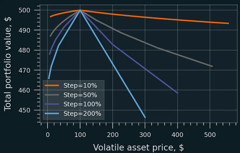
Smaller rebalancing steps reduce loss. Rebalancing costs and earned LP fees are excluded here. Initial asset price: $100, initial LP value: $200.
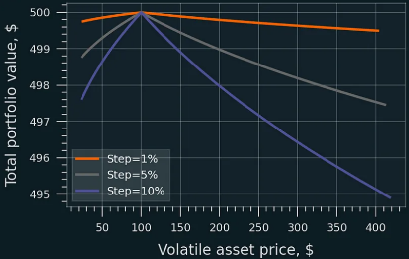
With very small steps, impermanent loss nearly vanishes. Costs and fees are not included. Same initial values.
The chart below estimates hedging costs via GBM simulation, assuming 0.3% swap fee, no trading fees. Even small rebalancing steps (1%-2%) incur low costs in Uniswap V2 full-range positions:
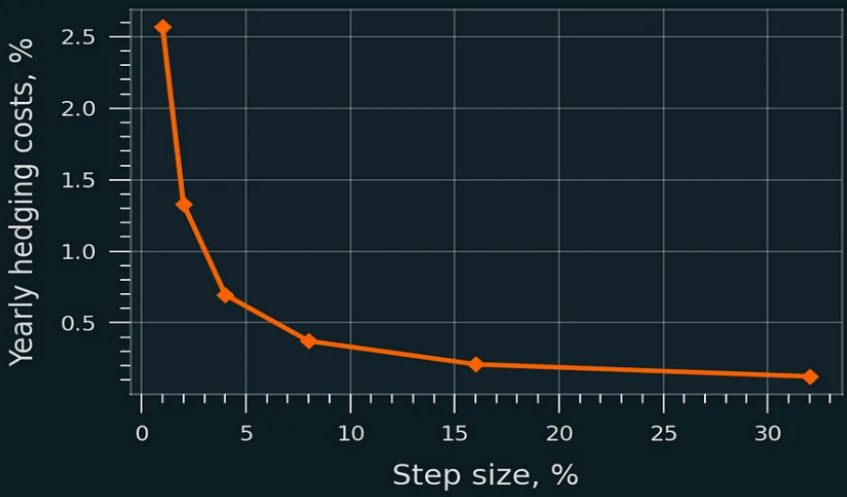
Annual swap cost of rebalancing as % of initial capital; Uniswap v2. Concentrated liquidity increases cost, yet remains small relative to capital:
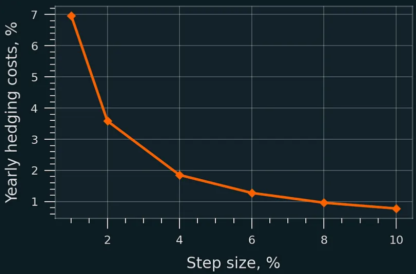
Annual rebalancing swap cost as % of initial capital; Uniswap v3; price range: [P/1.5, P*1.5], no liquidity migration.
So far, discussion focused on full-range delta-neutral strategies. But the same applies elsewhere. For instance, borrowing only 50% of volatile asset creates a hybrid: half follows √λ, half is delta-neutral.
Alternatively, borrow amount could be a function of price. Suppose initially LP borrows 100% of needed volatile asset, but gradually reduces it to zero as price rises. If price drops, reverse: borrow >100%, swap for stablecoins, deposit as collateral. This behavior forms a convex function:

Compared to HODL, partial and dynamic hedging. Step = 1%. Fees not shown.
Note: For Uniswap v3 positions with fixed price ranges, hedge rebalancing should coincide with liquidity relocation within the pool.
Key takeaways:
a. Through hedging and periodic rebalancing, LPs can protect capital against price swings. Delta-neutrality is achievable.
b. Using “x% price change” as a trigger minimizes divergence loss.
c. Smaller rebalancing steps reduce residual impermanent loss but increase hedging costs.
3.2 Power Perpetuals
Buying instruments with positive gamma: BiB Exchange introduces two tools—power perpetuals and options. We begin with power perpetuals.
Power Perpetuals: A newer concept where contract payoff scales with a power function (square, cube, etc.) of the underlying asset price. If ETH doubles:
- ETH² perpetual (e.g., Squeeth) quadruples
- ETH³ increases eightfold
- ETH⁵ increases 32-fold
Below compares returns of power perpetuals vs leveraged perps:
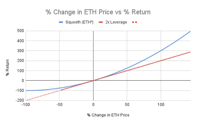
Squeeth offers higher upside than 2x leverage when price rises, lower drawdown when price falls.
Example:
Alice wants to hedge her full-range USDC/WETH LP position P. She consults the parameter table:
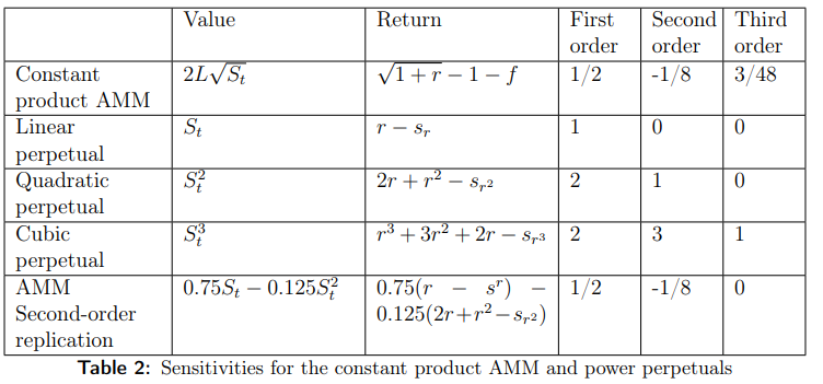
Explanation:
- Value: Portfolio value functions under different models
- Return: Payoff approximation using Taylor expansion, where r ≈ 0, and Sr, Sr², Sr³ denote funding rates for first-, second-, third-order power perps
- First, Second, Third Order: Coefficients in Taylor series expansion
Alice finds she needs a 50% short ETH and 12.5% long ETH² exposure (percentages derived from V(LP), total capital locked). She shorts ETH conventionally (via perp or borrowing), then buys Squeeth on Opyn or another power perp protocol. Squeeth ("squared ETH") is a derivative whose price tracks ETH².
If higher-order power perps were available, she might also go long 3/48×V(LP) ETH³ and short 15/384×V(LP) ETH⁴, etc.
To match a 50:50 HODL portfolio, she wouldn’t short ETH but directly buy 2nd+ order power perps (see figure):
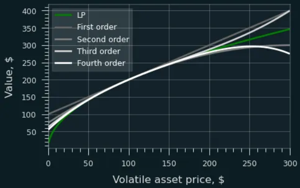
An LP’s value function can be approximated by a series of power perpetuals. Higher orders yield better accuracy.
The above figure shows how LP payoff can be fitted using power perpetuals. These require less frequent rebalancing—unlike linear hedges needing adjustment every 1%-5% move, even 50%-100% moves may suffice for adequate accuracy.
However, few protocols currently offer power perpetuals. Only Opyn’s Squeeth has gained traction, yet even it lacks deep liquidity. BiB Exchange concludes this method lacks practical viability today.
3.3 Options
1. Define Your Strategy Position:
Assume initial ETH price is $1000. Start with $1000 USDC (baseline). Sell 50% for ETH:
x₀ = 0.5 ETH
y₀ = 500 USDC
Provide 0.5 ETH and 500 USDC as liquidity in ETH-USDC pool.
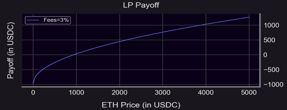
2. Calculate the Payoff Curve of the LP Position.
Uni V2 LP Value: V = 2*L*S^0.5 + fees
S = Spot price of ETH
L = (x₀ * y₀)^0.5
Subtract initial capital:
Profit = 2*L*S^0.5 + fees - 1000
For Uni V3, it's more complex:
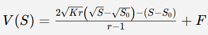
Where:
F = Cumulative fees;
K = (Upper price × Lower price)^0.5;
S₀ = Starting price;
r = (Upper / Lower)^0.5.
Larger r makes Uni V3 curve resemble Uni V2. Outside the range, payoff resembles options—suggesting hedging via options.
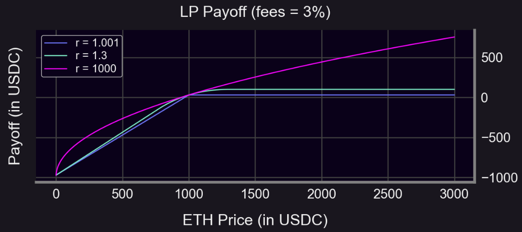
Initial ETH price = $1000
Buy 1 ATM put option (strike = $1000)
Put premium = $50
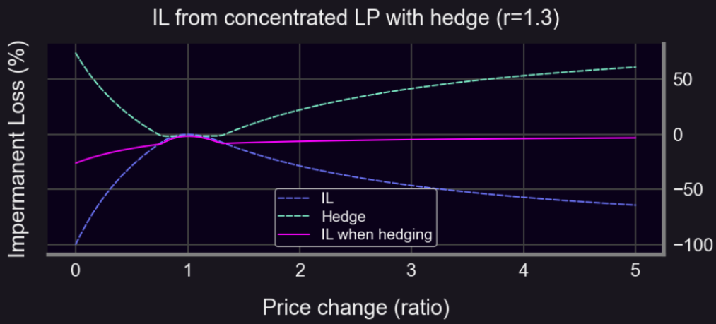
LP fees = 3% (r = 1.3, range: S₀/1.3 to S₀×1.3)
S < 1000: Hedged profit flatter (sometimes positive)
S ≥ 1000: Lower profit due to premium cost
Hedging always costs money. Must earn enough fees to cover premium.
Using 50:50 ETH-USDC as baseline, use a straddle to hedge:
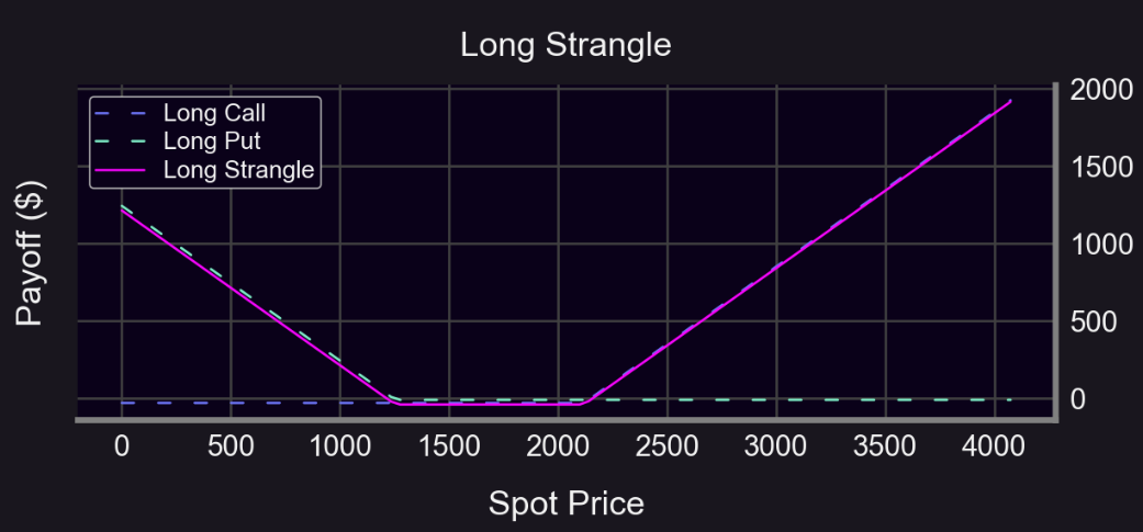
Clearly, a straddle limits impermanent loss even during sharp moves up or down:
Panoptic offers perpetual options for hedging. Users can hedge positions to reduce risk, while LPs provide required liquidity and earn fees. Panoptic’s perpetual options present another avenue for Uniswap hedging. BiB Exchange believes gamma hedging enables comprehensive risk management while leveraging the liquidity of perpetual structures.
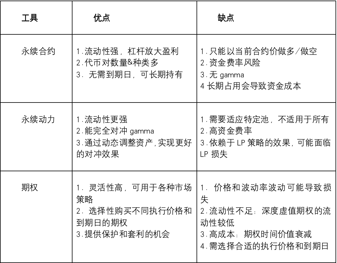
We summarize pros and cons of each hedging tool. Note: This is general comparison; actual performance depends on context and market conditions.
Conclusion
As shown, avoiding impermanent loss always incurs some trading cost. Balancing LP fees against hedging costs makes achieving ideal risk-free returns challenging. Each tool has trade-offs: perpetuals and power perpetuals offer strong liquidity but carry funding rate risks; options suffer from limited liquidity and high premiums.
BiB Exchange believes that in this evolving landscape of liquidity-driven financial innovation, hedging logic serves as both a guiding light and a powerful tool for scaling new financial heights. Investors must thoughtfully weigh LP fees against hedging costs, carefully choosing among tools to find the optimal strategy tailored to their needs.
Join TechFlow official community to stay tuned
Telegram:https://t.me/TechFlowDaily
X (Twitter):https://x.com/TechFlowPost
X (Twitter) EN:https://x.com/BlockFlow_News