

Vitalik: Exploring Elliptic Curve Pairings
TechFlow Selected TechFlow Selected
Vitalik: Exploring Elliptic Curve Pairings
Elliptic curves have been widely used for over three decades in cryptographic applications such as encryption and digital signatures.
Author: Vitalik Buterin
Published on: January 14, 2017
One of the key foundational primitives behind many cryptographic building blocks—such as deterministic threshold signatures, zk-SNARKs, and other simpler forms of zero-knowledge proofs—is elliptic curve pairings. Elliptic curves have been widely used in cryptography and digital signatures for over three decades. "Elliptic curve pairings" (also known as bilinear maps) are a recent extension built on top of elliptic curves that introduce cryptographic multiplication, greatly expanding what elliptic curve-based protocols can achieve. This article will explain elliptic curve pairings in detail and briefly describe how they work.
This concept is genuinely difficult, so don't expect to fully understand it even after reading this once or ten times. However, we hope this article can at least reveal some of its mysteries.
Elliptic curves themselves are already a challenging topic, but this article mostly assumes you have some understanding of their mechanics. If you lack basic familiarity, I recommend reading this primer first.
In summary, elliptic curves deal with mathematical objects called "points"—intuitively, points (x, y) on a two-dimensional plane—and special formulas for arithmetic operations like addition (e.g., computing R = P + Q). You can also multiply a point by an integer (e.g., P * n = P + P + … + P), though there's a much faster algorithm when n is large.
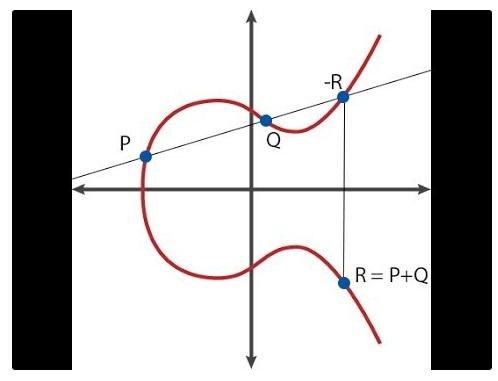
This illustrates what point addition looks like graphically
There is also a special point called the "point at infinity" (O), which acts as the zero element in point arithmetic—meaning P + O = P for any point P. A curve has a property called "order," meaning there exists a positive integer n such that P * n = O for all points P (and thus P * (n + 1) = P, P * ((7*n) + 5) = P * 5, etc.). Additionally, there is a pre-agreed "generator point" G—the point chosen to represent the unit element, analogous to the number 1. In theory, any point on the curve could serve as the generator, but it's crucial that G is uniformly selected.
Pairings allow you to verify more complex equations: for example, given P = G * p, Q = G * q, R = G * r, you can check whether p * q = r holds using only the coordinates of P, Q, and R. This may seem to break a fundamental security guarantee of elliptic curves, since knowing P's coordinates might appear to leak the value of p. But in reality, this leakage risk is very limited—in precise terms, the decisional Diffie-Hellman problem becomes easy, but the computational version remains "computationally infeasible." At minimum, solving it is no easier than without this capability.
A third way to understand pairings—one that may be most illuminating in many of the contexts we discuss—is to view elliptic curve points as outputs of a one-way encryption function (i.e., encrypt(p) = p * G = P). While traditional elliptic curve mathematics allows you to verify linear constraints between variables (e.g., verifying 5 * P + 7 * Q = 11 * R checks whether 5 * p + 7 * q = 11 * r), elliptic curve pairings enable verification of quadratic constraints (e.g., verifying e(P, Q) * e(G, G * 5) = 1 checks whether p * q + 5 = 0). The ability to handle quadratic relationships is sufficient to support interesting applications such as deterministic threshold signatures and QAPs (quadratic arithmetic programs, a form of zero-knowledge proof).
Now the question is: what exactly is this operation e(P, Q) we just introduced? This is what a "pairing" is. Mathematicians sometimes call it a "bilinear map," where "bilinear" essentially means it satisfies these conditions:
e(P, Q + R) = e(P, Q) * e(P, R)
e(P + S, Q) = e(P, Q) * e(S, Q)
Note that here "+" and "*" can be arbitrary operators. When defining new mathematical objects, abstract algebra doesn't care how "+" and "*" are defined, as long as they behave consistently with familiar rules like a + b = b + a, (a * b) * c = a * (b * c), and (a * c) + (b * c) = (a + b) * c.
If P, Q, R, S were just numbers, constructing such a pairing would be straightforward: we could define e(x, y) = 2^(xy). Then we’d see:
e(3, 4 + 5) = 2^(3 * 9) = 2²⁷
e(3, 4) * e(3, 5) = 2^(3 * 4) * 2^(3 * 5) = 2¹² * 2¹⁵ = 2²⁷
It really is bilinear!
However, such simple pairings aren't suitable for cryptography because analyzing mathematical objects operating directly on integers is trivial. Integer properties make operations like division and logarithms easy. Integers also lack concepts like "public keys" or "one-way functions." Moreover, the pairing described above is reversible: if you know x and e(x, y), you can compute y via division and logarithms. What we want is a mathematical structure as close to a "black box" as possible—you can perform certain additions, subtractions, multiplications, and divisions, but nothing else. This is where elliptic curves and elliptic curve pairings come into play.
It turns out that bilinear maps can indeed be constructed on elliptic curve points—that is, functions e(P, Q) mapping two points on an elliptic curve to an element in F_p¹² (sufficiently large in this specific case, though exact parameters vary depending on curve details, as mentioned later). However, the underlying mathematics is extremely complex.
First, let's introduce prime fields and extension fields. The pretty curves shown earlier assume the curve equation is defined over real numbers. But if we actually used real numbers in cryptography, someone could use logarithms to reverse-engineer secrets, rendering everything useless—and storing real numbers would require infinite space. Instead, we use numbers from finite fields.
A prime field consists of the set {0, 1, 2, ..., p−1}, where p is a prime, with arithmetic defined as follows:
a + b: (a + b) % p
a * b: (a * b) % p
a - b: (a - b) % p
a / b: (a * b^(p-2)) % p
Essentially, all operations are performed modulo p (here’s a primer on modular arithmetic). Division is special. Normally, 3/2 isn’t an integer, but we want to work only with integers, so instead we find an integer x such that x * 2 ≡ 3 mod p, where multiplication is the modular multiplication defined above. Fortunately, thanks to Fermat's Little Theorem, this exponentiation formula works, though a faster method is the extended Euclidean algorithm. Let p = 7; here are some examples:
2 + 3 = 5 % 7 = 5
4 + 6 = 10 % 7 = 3
2 - 5 = -3 % 7 = 4
6 * 3 = 18 % 7 = 4
3 / 2 = (3 * 2^5) % 7 = 5
5 * 2 = 10 % 7 = 3
If you experiment with these operations, you’ll find they’re consistent and satisfy all usual algebraic rules. The last two examples show (a / b) * b = a. You can also verify (a + b) + c = a + (b + c), (a + b) * c = a * c + b * c, and other algebraic identities you learned in high school continue to hold. In practical elliptic curves, points and equations are typically defined over prime fields.
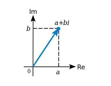
Now let’s discuss extension fields. You may have encountered them before—the most common example in math textbooks being the complex numbers, formed by extending the real numbers with a new element sqrt(-1) = i. Broadly speaking, an extension field is created by introducing a new element to an existing field and defining its relationship to existing elements (in this case, i² + 1 = 0); this relation must not be satisfiable by existing elements. The resulting structure is the set of all linear combinations of the original elements plus the new one.
We can extend prime fields similarly. For example, adding i to the prime field modulo 7 gives us:
(2 + 3i) + (4 + 2i) = 6 + 5i
(5 + 2i) + 3 = 1 + 2i
(6 + 2i) * 2 = 5 + 4i
4i * (2 + i) = 3 + i
The last equation may be harder to follow. First distribute: 4i * 2 + 4i * i = 8i - 4. Working modulo 7, this becomes i + 3. For division:
a / b : (a * b^(p^2-2)) % p
Here, Fermat's Little Theorem uses exponent p² instead of p (though the extended Euclidean algorithm can still be used more efficiently). Since every element x in the field satisfies x^(p² − 1) = 1, we call (p² − 1) the "order of the multiplicative group of the field."
For real numbers, the fundamental theorem of algebra guarantees that its quadratic extension—the complex numbers—is algebraically closed: no further extensions are possible because any new element j satisfying polynomial relations with existing complex numbers already has a solution within the field. But prime fields don’t have this limitation—we can perform cubic extensions (where a new element w satisfies a cubic polynomial, making 1, w, w² linearly independent), higher-degree extensions, or even iterated extensions. Elliptic curves used in cryptography are built over such modular "complex numbers."
For those interested in implementing these math structures in code, here are examples of implementations for prime and extension fields.
Back to elliptic curve pairings. An elliptic curve pairing (one specific type among others, though the logic is similar) is a mapping G2 × G1 → Gt, where:
- G1 is an elliptic curve whose points satisfy equations of the form y² = x³ + b, with x, y coordinates in F_p (ordinary integers under modular arithmetic with a prime modulus).
- G2 is another elliptic curve satisfying the same equation, but with x, y coordinates in F_p¹² (the "complex numbers" discussed earlier; we define a magic number w satisfying a 12th-degree polynomial w¹² − 18w⁶ + 82 = 0).
- Gt is the target group—the codomain of the pairing. In our case, Gt is F_p¹² (using the same "complex numbers" as G2).
The main required property is bilinearity, which in this context means:
e(P, Q + R) = e(P, Q) * e(P, R)
e(P + Q, R) = e(P, R) * e(Q, R)
(Note: Strictly speaking, this is "bilinearity over ℤ"—since all points on the elliptic curve are integer-coordinate points and operations are defined as integer arithmetic followed by modular reduction, certain linearity properties naturally hold.)
Two additional criteria for choosing a pairing function:
- Efficiency (e.g., we could take discrete logs of all points and multiply them—a trivial pairing method—but this requires solving ECDLP, which defeats the purpose)
- Non-degeneracy (defining e(P, Q) = 1 is trivial but useless)
So how do we achieve this?
The mathematics enabling pairing functions is highly advanced and goes beyond what we've seen so far, but here's a rough outline. We first need to define the concept of a "divisor," which is essentially another way to represent functions acting on elliptic curve points. A divisor of a function counts its zeros and poles (points where it goes to infinity). To clarify, consider some examples. Fix a point P = (P_x, P_y) and examine this function:
f(x, y) = x − P_x
Its divisor is [P] + [−P] − 2 * [O] (square brackets denote membership in the multiset of zeros and poles, not the point itself; [P] + [Q] ≠ [P + Q]). Why?
- The function is zero at P because x = P_x ⇒ x − P_x = 0
- The function is zero at −P because −P shares the same x-coordinate as P
- As x approaches infinity, the function does too—so we say it has a pole at O. This pole counts twice, hence multiplied by −2 (negative because it's a pole, 2 because it occurs twice).
Computationally, since the curve equation is x³ = y² + b, as x grows, y must grow roughly 1.5 times faster to maintain balance. Thus, a linear function in x alone has multiplicity 2 at infinity; if it includes y, multiplicity becomes 3.
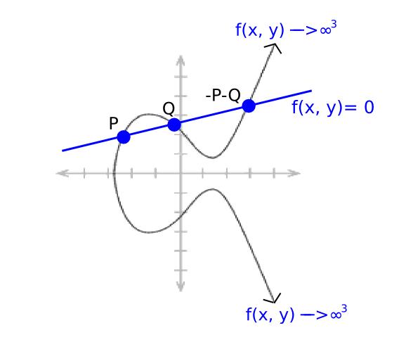
Now consider a linear function:
ax + by + c = 0
Choose a, b, c so the line passes through points P and Q. By elliptic curve addition rules, it must also pass through −P−Q. Since it depends on both x and y as it approaches infinity, its divisor is [P] + [Q] + [−P−Q] − 3 * [O].
We know that every "rational function" (defined via finite additions, subtractions, multiplications, and divisions of point coordinates) corresponds uniquely to a divisor up to a constant multiple (i.e., if two functions F and G have the same divisor, then F = k*G for some constant k).
For any two functions F and G, the divisor of (F * G) equals the sum of their divisors (in textbooks: (F * G) = (F) + (G)). For example, if f(x, y) = P_x − x, then (f³) = 3*[P] + 3*[−P] − 6*[O]; P and −P count thrice because f³ approaches zero "three times faster" in a precise mathematical sense.
Note a theorem: if you remove the brackets from a divisor and sum the points using elliptic curve arithmetic, the result must be O (e.g., [P] + [Q] + [−P−Q] − 3*[O] evaluates to P + Q − P − Q − 3*O = O). Any divisor with this property corresponds to some function.
Now we approach the Tate pairing. Consider functions defined by these divisors:
- (F_P) = n * [P] − n * [O], where n is the order of G1 (so n * P = O for all P)
- (F_Q) = n * [Q] − n * [O]
- (g) = [P + Q] − [P] − [Q] + [O]
Now consider the product F_P * F_Q * g^n. Its divisor is:
n * [P] − n * [O] + n * [Q] − n * [O] + n * [P + Q] − n * [P] − n * [Q] + n * [O]
Simplifying yields neatly:
n * [P + Q] − n * [O]
Notice this matches the divisor form of F_P and F_Q. Hence F_P * F_Q * g^n = F_(P + Q).
Next, apply a step called "final exponentiation": raise the previous result (F_P, F_Q, etc.) to the power z = (p¹² − 1) / n, where p¹² − 1 is the order of the multiplicative group in F_p¹² (i.e., x^(p¹² − 1) = 1 for all x ∈ F_p¹²). Note that applying this exponent to any result already raised to the n-th power yields something to the (p¹² − 1)-th power, which equals 1. Thus, after final exponentiation, g^n cancels out, giving F_P^z * F_Q^z = F_(P + Q)^z—establishing part of bilinearity.
To construct a function bilinear in both arguments, heavier mathematics is needed—going beyond just computing F_P to analyzing its divisor leads to the full Tate pairing. Proving deeper results requires concepts like "linear equivalence" and Weil reciprocity. Detailed treatments can be found here and here.
An optimized variant of the Tate pairing—the Optimal Ate Pairing—has been implemented. The code also implements Miller's algorithm to compute F_P.
Using such pairings is a double-edged sword: while they enable powerful new protocols, they also demand extra caution when selecting elliptic curves.
Every elliptic curve has an "embedding degree" k—the smallest integer such that p^k − 1 is divisible by n (p is the field prime, n the curve order). In our earlier example, k = 12. In traditional elliptic curve cryptography (where pairings are irrelevant), embedding degrees are typically huge—making pairing computation computationally infeasible. But careless construction might yield k = 4 or even k = 1.
When k = 1, the elliptic curve "discrete logarithm problem" (finding p given only P = G * p—the task required to break EC private keys) reduces to a relatively easy problem over F_p (via the MOV attack). Using curves with embedding degree ≥12 ensures such reductions are impossible—or result in problems no easier than solving ECDLP directly. All standard curve parameters today are carefully vetted to avoid this issue.
Join TechFlow official community to stay tuned
Telegram:https://t.me/TechFlowDaily
X (Twitter):https://x.com/TechFlowPost
X (Twitter) EN:https://x.com/BlockFlow_News